Calculations

Probability of failure can be calculated for all Distribution models. The GE Digital APM system uses the following formula to determine failure probability:

Where:

• P(t1|t0) is the failure probability at any given time assuming that the equipment has not yet failed at the current age. If you specify a failure probability, the GE Digital APM system will use this value to calculate the future age of the equipment.
• D(t) is the cumulative distribution function, or the failure probability at time t for a new piece of equipment. The curve in the CDF plot represents this function.
• t0 is the current age of the piece of equipment.
• t1 is the future age of the piece of equipment. If you specify an operating time, this value is determined by adding the time to the current age of the piece of equipment, and the resulting value is then used to calculate the failure probability.
• n is the number of subcomponents the piece of equipment contains (e.g., tubes in a heat exchanger bundle). If the failure type of the Reliability Distribution Analysis is Failure with replacement, the number of subcomponents is 1. If the failure type is Failure without replacement, this value is mapped from a query or dataset or manually entered when you create the Reliability Distribution Analysis.

A Goodness of Fit (GOF) test determines how well your analysis data fits the calculated data model.

• If your data passes the GOF test, your data follows the data model closely, and you can rely on the predictions made by model.
• If your data fails the GOF test, it may not follow the model closely enough to confidently rely on model predictions.

On the Reliability Growth page, in the Segment pane, the Passed GOF check box is selected when your data passes the test and cleared when your data fails the test.

To determine whether the data passes the GOF test, the GE Digital APM system uses the following values:

• GOF Statistic: Determines how precisely the data fits the model. This value is calculated from a Cramer-von Mises or Chi-squared test and is displayed in the GOF Statistic column in the Segment pane on the Reliability Growth page.
• Alpha Value: Determines what critical value to use for the GOF test. This value depends on the Confidence Level you select for the analysis.
• Critical Value: Determines whether the data passes the GOF test. This standard value depends on the number of datapoints included in the analysis and the alpha value. It is displayed in the Critical Value column in the Segment pane on the Reliability Growth page.

Test Statistics

GE Digital APM uses two different methods to calculate GOF for Reliability Growth Analyses, depending on whether or not the analyses use grouped data.

Goodness of Fit (GOF) for a Reliability Growth Analyses based on data that is not grouped is calculated using the Cramer-von Mises test.

For analyses whose end date is time-based, Cramer-von Mises test uses the following formula to calculate the GOF Statistic:

For analyses whose end date is event-based, Cramer-von Mises test uses the following formula to calculate the GOF statistic:

Goodness of Fit for a Reliability Growth Analysis based on grouped data is calculated using a Chi-squared test. This test uses the following formula to calculate a test statistic:

Critical Value: Cramer-von Mises Test

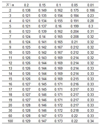
For non-grouped data, the Cramer-von Mises test is used to determine whether the data passes the GOF test. This test compares the GOF Statistic to a Critical Value. The Critical Value depends on two values:

• Alpha = 1- Confidence Level
• N = The number of datapoints in the population.

Alpha is determined using the Confidence Level, which you can define manually for each analysis. The Confidence Level indicates the percentage of uncertainty of the Goodness of Fit method. This percentage is usually determined by experience or an industry standard and limits how closely the data must fit the model in order for it to pass the Goodness of Fit test. The higher the Confidence Level, the easier it will be for your data to pass the Goodness of Fit test. The lower the Confidence Level, the harder it will be for your data to pass the Goodness of Fit test. If the data does pass, however, the data will be a very close fit to the model.

After a Confidence Level has been determined, the GE Digital APM system uses the following Critical Values for Cramer-von Mises Test chart to find the Critical Value. The chart displays critical values at five confidence levels (80%, 85%, 90%, 95% and 98%) which in turn calculate 5 alpha values (0.2, 0.15, 0.1, 0.05, 0.02).

Critical Value: Chi-squared Test

For grouped data, the Chi-squared test is used to determine whether the analysis passed the GOF test. This test uses Degrees of Freedom (i.e., the number of datapoints - 2) and the Confidence Level to calculate a Critical Value, which is then compared to the GOF Statistic to determine whether the analysis passed the GOF test. The Confidence Level is defined the same way it is in the Cramer-von Mises test (i.e., it indicates the percentage of uncertainty of the Goodness of Fit method).

The following formula is used to calculate the Chi-squared distribution.

In the formula, k is degrees of freedom and F(x;k) is the Confidence Level. These values are used to find the Critical Value, x.

Determining the Results

For both the Cramer-von Mises test and the Chi-squared test, if the GOF statistic is greater than the Critical Value at the chosen Confidence Level, the data fails the GOF test. This means the data does not follow the analysis pattern closely enough to confidently predict future measurements. If the GOF Statistic is lower than the Critical Value, the population passes the test, which means data is more likely to occur in a pattern and therefore is more predictable.

For example, if you run a Reliability Growth Analysis on a set of failure data, and the data fails the GOF test, it may mean that the piece of equipment or location does not fail in a predictable pattern (i.e., the piece of equipment or location fails at random). If this is the case, any predictions you make based on this data will not be as reliable as predictions made against data that has passed the GOF test.

If the analysis fails a GOF test, it does not necessarily mean that you cannot use the data model. The Reliability Growth Analysis might fail a GOF test because there is more than one trend within the data. If you suspect this is the case, you can split the analysis into segments at the points where it looks like a change occurred. Afterwards, the separate segments may individually pass the GOF test because they have been split up into multiple failure patterns.

Additionally, if the analysis fails the GOF test, you should also check for a visual goodness of fit. Models can sometimes still be used even if the analysis does not pass the GOF test.

Failure Rate

Grouped Data

MTBF

Cumulative Failures

Non-grouped Data

Time-Terminated

The parameters λ and ß are estimated using the following equations:

where, the unbiased ß estimate is .

Where,

• N is the number of observations.
• T is the total time of observation.
• Xi is the cumulative failure times.

Failure-Terminated

The parameters λ and ß are estimated using the following equations:

, where, the unbiased ß estimate is .

Where,

• N is the number of observations.
• T is the total time of observation.
• Xi is the cumulative failure times..

MLE

Where, is the failure time (in t-space) of component i, i=1,..., r or the censoring time (in t-space) of component i, i=r+1,..., n. If there is no censoring (complete data), r = n and the last term in the Likelihood function disappears. The terms and are the standard normal probability density and standard normal cumulative distribution.

Least Square

Let us denote : n = total cases, r = uncensored cases, and n - r = k = censored cases

If ,, then the parameters for are estimated using the following equations:

In this case, and .

Failure Rate

PDF

CDF

Reliability

MLE

Where, is the failure time of component i, i=1,..., r or the censoring time of component i, i=r+1,..., n. If there is no censoring (complete data), r = n and the last term in the Likelihood function disappears.

Least Square

Suppose, and

Using these transformed data, we can obtain the parameter estimate using the following equation:

R-Squared

If and , then the parameters for are estimated using the following equations:

Kolmogorov-Smirnov Test

• Calculating modified failure order for sample dataset

  

  

  Where,

  • Oj is the order of the jth failure
  • Ij is the increment for the jth failure
  • n is the total number of data points, both censored and uncensored
  • Op is the order of previous failure
  • c is the number of data points remaining in the data set, including the current data point
  Note: When there are no censored data, the above equation can be simplified to Oj = j.

• Calculating median rank from modified failure order

  Median rank is the median value of the rank distribution. Rank distribution is the distribution of the probability of j^th ordered value x out of a sample n.

  

  Incomplete beta function is used to find median rank of the above equation

  

• Finding statistics of the KS test

  Statistics refers to the maximum difference between median rank calculated from dataset and probability calculated from the reference distribution. This steps does not considers the censored data.

  

• Calculating p-value from KS test statistics and sample size

  

  Where,

• Calculating significant level (alpha)

  alpha = 1-confidence level

• Failing the Goodness of Fit test

  If the p-value <= alpha, Goodness of Fit test fails because there is statistically significant difference between the sample dataset and the reference distribution.

Failure Rate

PDF

CDF

Reliability

MLE

Where, is the failure time (in t-space) of component i, i=1,..., r or the censoring time (in t-space) of component i, i=r+1,..., n. If there is no censoring (complete data), r = n and the last term in the Likelihood function disappears. The terms and are the standard normal probability density and standard normal cumulative distribution.

Least Square

Let us denote : n = total cases, r = uncensored cases, and n - r = k = censored cases

If ,, then the parameters for are estimated using the following equations:

In this case, and .

Failure Rate

PDF

CDF

Reliability

MLE

Where, is the failure time of component i, i=1,..., r or the censoring time of component i, i=r+1,..., n. If there is no censoring (complete data), r = n and the last term in the Likelihood function disappears. The terms and are the standard normal probability density and standard normal cumulative distribution.

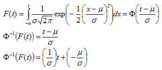
Least Square

Let us denote : n = total cases, r = uncensored cases, and n - r = k = censored cases

If and , then the parameters for are estimated using the following equations:

In this case, and .

Risk Properties

• PF Interval: The time period before a failure in which a potential failure could be detected.
• Repair Immediately: If this field value is True, then you should trigger a planned correction immediately to fix the potential failure if a potential failure is detected in advance. Otherwise, wait until the value in the Percentage of PF Interval to Wait (%) field reaches 0.
• Percentage of PF Interval to Wait (%): A numeric value that indicates how long to wait to repair the piece of equipment or location, presented as a percentage of the PF Interval value.

Inspection Properties

• Detection Probability (%): The probability of finding potential failures when the monitored risk is in its PF interval. The simulation engine randomly determines whether a potential failure could be detected according to the Detection Probability. The inspection will notify the simulation engine once a potential failure is determined to be detectable.

Condition Monitor Properties

• Detection Probability (%): The probability of finding potential failures when the monitored risk is in its PF Interval. The simulation engine randomly determines whether a potential failure could be detected according to the Detection Probability. The inspection will notify the simulation engine once a potential failure is determined to be detectable. This is randomly chosen and evenly distributed in the PF Interval of the risk.

Failure Rate

PDF

CDF

MLE

Where is the failure time of component i, i=1,..., r or the censoring time of component i, i=r+1,..., n. If there is no censoring (complete data), r = n.

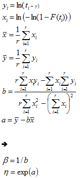
Least Square