Probability Distribution Analysis

About Probability Distribution Analysis

Probability Distribution Analysis allows you to describe the Time to Failure (TTF) as a statistical distribution, which usually is characterized by a specific pattern.

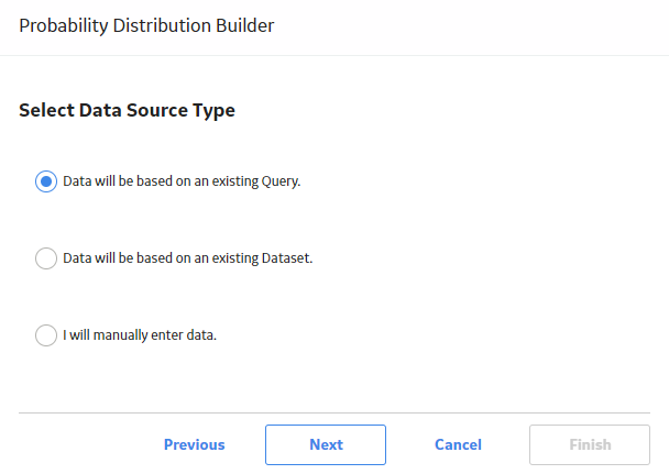
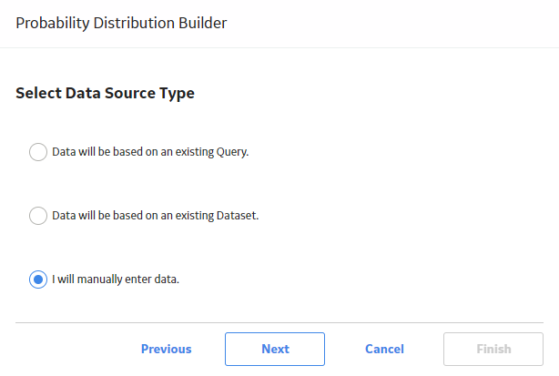
Based on a query, dataset, or data that you manually enter, you can use an independent variable to generate a Probability Distribution Analysis. GE Digital APM Reliability supports four Distribution types:

About Data Censoring in a Probability Distribution Analysis

Probability Distribution Analysis supports the functionality of censoring, which accounts for the period of time from the last failure date to the analysis end date. You can censor or ignore datapoints in a Probability Distribution Analysis to estimate the probability when a failure might occur. Censoring is based on failure modes.

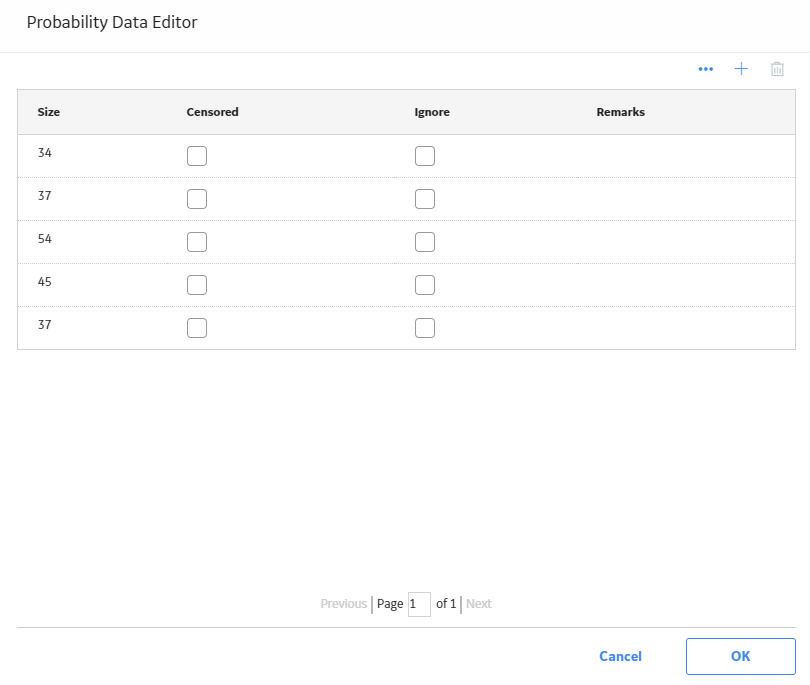
Censoring a datapoint means that the datapoint is excluded as a failure but included in the operating time of the Asset. If you select the Censored check box, the data in the selected row is excluded. When you create a Probability Distribution Analysis using a query or dataset as the data source, the GE Digital APM system automatically censors time values from the beginning of the Analysis Period to the first event and the time value from the last event to the end of the analysis. After the calculations for the analysis have been performed, each time that the query or dataset is refreshed, the failure data will be automatically censored.

Regardless of the data source you use, you can censor any failure data. Consider the following:

For Maximum Likelihood Estimators (MLE), the maximum number of censored datapoints is one (1) less than the total number of datapoints.
For Least Squares estimation, the maximum number of censored datapoints is two (2) less than the total number of datapoints.

Pump Failure

Assume that you want to determine the reasons for a pump failure.

A pump might have failed due to multiple reasons, such as rusted part, motor overheating, insufficient power supply, or power outage. Each of these reasons will have its own specific failure rate and probability density function. To determine the failure rate of "motor overheating," you must censor all other failure modes from the analysis.

Further, motor overheating might be caused due to multiple reasons, such as improper operation, improper application, and improper maintenance. The censoring feature allows you to separate the failure modes, and determine which is the dominant failure mode. Based on this information, you can decide what is needed to improve the motor performance.

Access a Probability Distribution Analysis

Procedure

Access the RA Overview page.
Select the Probability Distribution tab.

A list of Probability Distribution Analyses available in the database appears.
Select the Probability Distribution Analysis whose details you want to view.
The Analysis Summary workspace for the selected analysis appears, displaying a preview of the Probability Distribution Function (PDF) plot and the Cumulative Density Function (CDF) plot. The workspace also contains the following sections at the bottom of the workspace:
- Distribution Options : Contains the summary of distribution properties for the selected Probability Distribution Analysis and allows you to modify these properties.
- Distribution Parameters: Contains the distribution parameters, which are determined by the distribution type.
- Goodness of Fit Test: Displays the results of the Goodness of Fit (GOF) test and includes the Statistic, P-Value and Passed fields.
The left pane contains the following tabs:

About Probability Plot

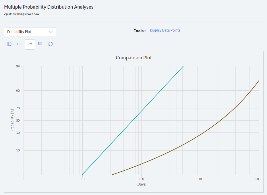
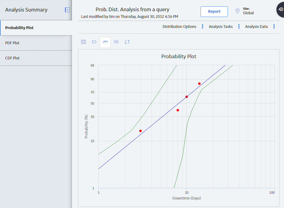
The Probability Plot is a log-log plot with data overlay and confidence limits that graphically displays the probability (expressed as a percentage) of each possible value of the random variable (CDF Occurrence % vs. time). CDF Occurrence % used here is numerically equal to the value from the cumulative distribution.

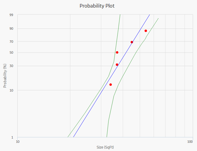
Note: Time used here refers to life data, not calendar data.

The Probability Plot shows the same data as the CDF plot, just represented in a log-log format. The log-log format reflects the standard technique for representing Weibull Distribution. Log-log format Data overlay gives a visual estimate of Goodness of Fit (GOF). Data overlay also gives clues to the presence of multiple failure modes. If a single or multiple inflection points exist in the data, then there is a possibility of multiple failure modes.

Note: Interaction with charts is not available on touch-screen devices.

Graph Features

While accessing a Probability Plot, you can:

Hover or tap on any datapoint to view the coordinates and the details of a datapoint.
- For an Estimated datapoint, you can view the type of distribution, the distribution parameters, and the value of R-Squared.
- For an Observed datapoint, you can view the name and the value of Variable.
Click or double-tap on any observed datapoint to view the data on the Distribution Data window.
Censor a datapoint.
Customize the appearance of the plot by using standard graph features.
Customize the data displayed in the graph by adjusting the x-axes to vary the display range.

About PDF Plot

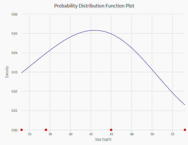
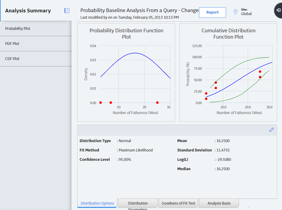
The Probability Density Function (PDF) plot is a lin-lin plot that counts the number of failures (or any other data) between certain time periods, creating a curve fit that estimates how many failures (failure data or any other data) you can expect to occur at a given point of time. This plot shows Density vs. Size. The term Density is used here with failure data to describe the size of the population that failed at the particular value of size (SqFt). A PDF plot helps you to answer a question such as, "What is the chance of a member of the population failing at exactly the time in question?"

Note: Interaction with charts is not available on touch-screen devices.

Graph Features

While accessing a PDF plot, you can:

Hover or tap on any datapoint to view the coordinates and the details of a datapoint.
- For an Estimated datapoint, you can view the type of distribution, the distribution parameters, and the value of R-Squared.
- For an Observed datapoint, you can view the name and the value of Variable.
Click or double-tap on any observed datapoint to view the data on the Distribution Data window.
Censor a datapoint.
Customize the appearance of the plot by using standard graph features.
Customize the data displayed in the graph by adjusting the x-axes to vary the display range.

About CDF Plot

The Cumulative Distribution Function (CDF) plot is a lin-lin plot with data overlay and confidence limits. It shows the cumulative density of any data set over time (i.e., Probability vs. size). The term Probability is used in this instance to describe the size of the total population that will fail (failure data or any other data) by size (SqFt).

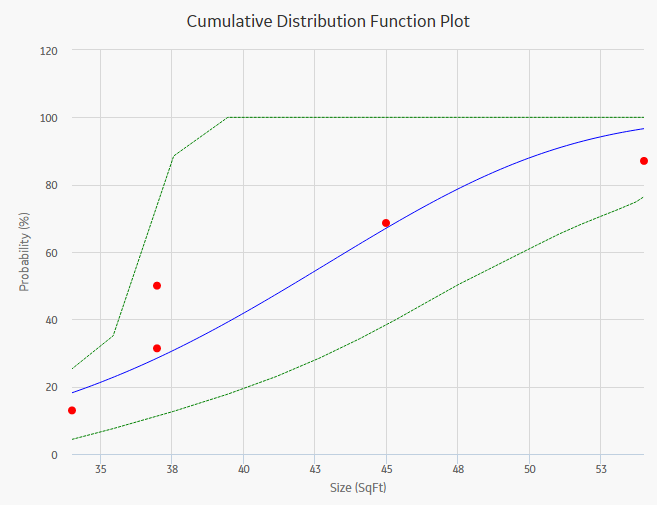
CDF plot answers a different question than PDF. For example, "What is the probability of failure at Size (SqFt)?" The CDF curve is the area under the PDF curve. The CDF accumulates all probability of failure up to the point in time in question. Since the number of failures increases with increasing size, the slope of the curve is always positive, always increasing.

Note: Interaction with charts is not available on touch-screen devices.

Graph Features

While accessing a CDF plot, you can:

Hover or tap on any datapoint to view the coordinates and the details of a datapoint.
- For an Estimated datapoint, you can view the type of distribution, the distribution parameters, and the value of R-Squared.
- For an Observed datapoint, you can view the name and the value of Variable.
Click or double-tap on any observed datapoint to view the data on the Distribution Data window.
Censor a datapoint.
Customize the appearance of the plot by using standard graph features.
Customize the data displayed in the graph by adjusting the x-axes to vary the display range.

Collect Data for Probability Distribution Analysis

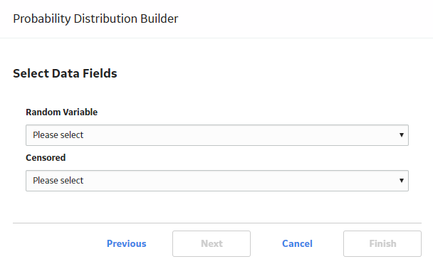
To create a Probability Distribution Analysis, you must select the field that contains the value that you want to analyze.

The following table shows the typical data needed to build and analyze Probability Distribution Analyses.


Data Required	Data Type	Description	Behavior and Usage
Censored	Logical	As needed, select the field to provide censoring information. Select the field from the data source that contains a value that indicates censored values.	This field is optional.
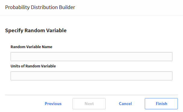
Random Variable	Character	If the data source is a query, the name of the random variable and the units of measure will be pre-populated based on the selection you made in the Value field on the previous screen. If you selected a different data source, type the name of the random variable in the Random Variable field and the units of measure for the random variable in the Units field.	This field is optional.
Units	Character	Select the units of measure for the random variable.	This field is optional.
Value	Numeric	Select the field that contains the value you want to analyze.	This is a required field.

Access Multiple Probability Distribution Analyses

About this task

You can access multiple Probability Distribution Analyses and compare multiple plots for the selected analyses. You cannot modify the details of the analyses based on which the Comparison Plot is generated.

Procedure

Access the RA Overview page.
Select the Probability Distribution tab.

A list of Probability Distribution Analyses available in the database appears.
Select two or more Probability Distribution Analyses whose plots you want to compare.

Note: You can select up to 20 analyses to compare plots.
In the upper-right corner of the grid, select .
The Multiple Probability Distribution Analysis page appears, displaying the Comparison Plot. By default, Probability Plot for the selected analyses appears. You can also view the following types of plots:
- PDF plot
- CDF plot

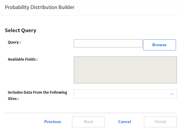
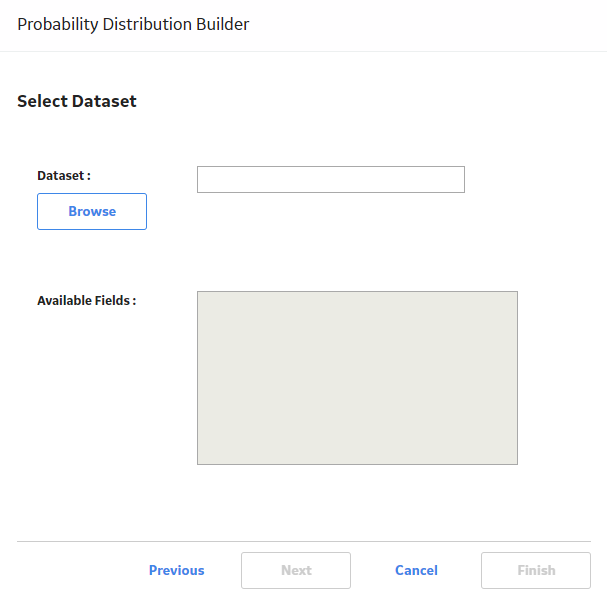
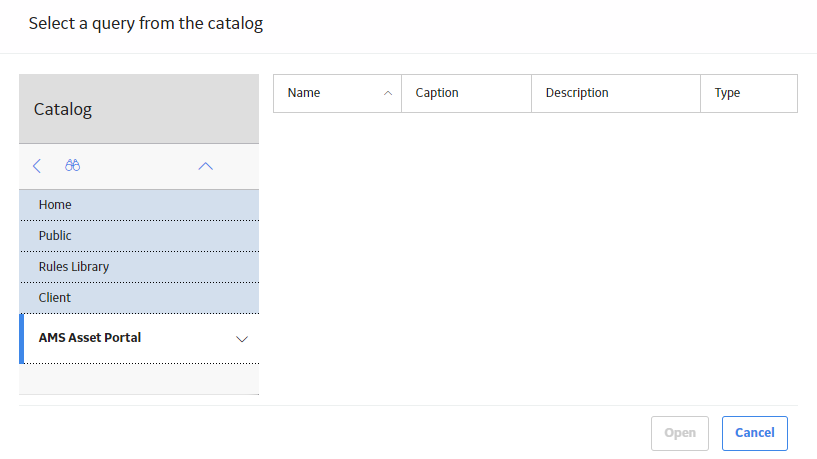
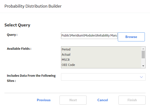
Create a Probability Distribution from an Existing Query or Dataset

Procedure

Access the RA Overview page.
In the upper-right corner, select New Analysis, and then select Probability Distribution.

The Probability Distribution Builder window appears, displaying the Define New Analysis screen.

Note: All required information is provided, but for additional information, consult the Distribution Analysis Families topic.
Enter values in the Analysis Name and Description boxes for the new analysis, and then select Next.

The Select Data Source Type screen appears. The Data will be based on an existing Query option is selected by default.
If you want to load data using an existing query, select Next.

The Select Query screen appears.

-or-

If you want to load data using an existing dataset, select Data will be based on an existing Dataset, and then select Next.

The Select Dataset screen appears.
Select Browse to search for an existing query or dataset in the GE Digital APM Catalog.

The Select a query from the catalog or Select a dataset from the catalog window appears, depending on whether you selected Data will be based on an existing Query or Data will be based on an existing Dataset in the previous step.

The following image shows the screen to select a query:
Select the required query or dataset, and then select Open.

The complete path to the query or dataset is displayed in the Query or Dataset box. The fields that exist for the selected query or dataset appear in the Available Fields list.

The following image shows the path to a selected query and the fields in the Available Fields list:
In the Includes Data From the Following Sites list, select the site(s) whose data from which you want to create an analysis.
If you are creating an analysis in a database that has only one site stored in the Site Reference family, then the Includes Data From the Following Sites list will not appear on the Select Query screen.
Select Next.

The Select Data Fields screen appears.
As necessary, specify values in the following fields:
1. In the Random Variable list, select a numeric value. This is a required field. A random variable associates a numerical value with every event. It describes a (possibly infinite) set of different events having a related probabilistic structure. The probability distribution of the random variable is a function that maps each possible value of the random variable to a particular probability.
2. In the Censored list, select a field that indicates censored values (i.e., not included in the Probability Distribution Analysis calculations). The selected field must be a logical field. This is an optional field.
Select Next.

The Specify Random Variable screen appears.
In the Random Variable Name box, enter the name of the random variable.
In the Units of Random Variable box, enter the units of measure for the random variable selected above.
Select Finish.

The GE Digital APM system generates the analysis and the Probability Distribution page appears, displaying the analysis results.

Create a Probability Distribution from Manually Entered Data

Procedure

Access the RA Overview page.
In the upper-right corner, select New Analysis, and then select Probability Distribution.

The Probability Distribution Builder appears, displaying the Define New Analysis screen.

Note: All required information is provided, but for additional information, consult the Distribution Analysis Families topic.
Enter values in the Analysis Name and Description boxes for the new analysis, and then select Next.

The Select Data Source Type screen appears.
Select I will manually enter data, and then select Next.

The Select Data Format screen appears.
In the Random Variable Name box, enter the name of the Random Variable.
In the Units of Random Variable box, enter the units of measure for the Random Variable selected above.
Select Finish.

The Probability Distribution Data Editor window appears.
Enter the information about the random variables that you want to include in the analysis. By default, the following columns are listed on the grid:
- Random Variable : Provide the value of the random variable.
- Censored : Select the check box to censor data.
- Ignore : Select the check box if you do not want to include the data on the selected row in the calculations.
- Remarks : Provide comments about the event.
Note: A minimum of three failure data points are needed to perform a calculation or you will receive a warning message and the analysis will not be generated.

Tip: You can add more rows of data by selecting Add at the bottom of the grid. You can remove any row of data by selecting the Remove next to the row of data that you want to delete.
Select OK.

The GE Digital APM system generates the analysis. The Distribution Data window closes and the Probability Distribution page appears, displaying the analysis results.

Change the Distribution Type of a Probability Distribution Analysis

About this task

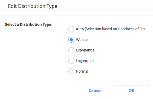
When you create a Probability Distribution Analysis, the Distribution Type is set to Weibull by default. After the analysis is created, you can change the Distribution Type to one of the following:

Normal
Weibull
Exponential
Lognormal
Triangular
Gumbel
Generalized Extreme Value
Auto

Note: Select Auto if you want the GE Digital APM system to select the appropriate Distribution Type based on the results of the Goodness of Fit test.

You can change the Distribution Type from the Analysis Summary workspace or from any of the plot tabs in the left pane.

Procedure

Access a Probability Distribution Analysis for which you want to modify the Distribution Type.
If you want to change the Distribution Type from the Analysis Summary workspace:
1. In the bottom section, select Distribution Options, and then select .
  The Distribution Type field is enabled.
2. In the Distribution Type box, select the desired Distribution Type, and then select .
  The analysis is recalculated based on the selected Distribution Type.
-or-

If you want to change the Distribution Type from one of the plot tabs (e.g., Probability Plot tab):
1. In the left pane, select the Probability Plot tab.
  The Probability Plot appears in the workspace.
  
  Note: You can also change the Distribution Type via the PDF Plot or CDF Plot tabs.
2. In the upper-right corner of the workspace, select Distribution Options, and then select Distribution Type.
  The Edit Distribution Type window appears.
3. Select the desired Distribution Type, and then select OK.
  The analysis is recalculated based on the selected Distribution Type.

About Normal Distribution

A Normal Distribution describes the spread of data values through the calculation of two parameters: mean and standard deviation. When using the Normal Distribution on time to failure data, the mean exactly equals MTBF and is a straight arithmetic average of failure data. Standard deviation (denoted by sigma) gives estimate of data spread or variance.

A Normal Distribution uses the following parameters:

Mean: The arithmetic average of the datapoints.
Standard Deviation: A value that represents the scatter (how tightly the datapoints are clustered around the mean).

About Weibull Distribution

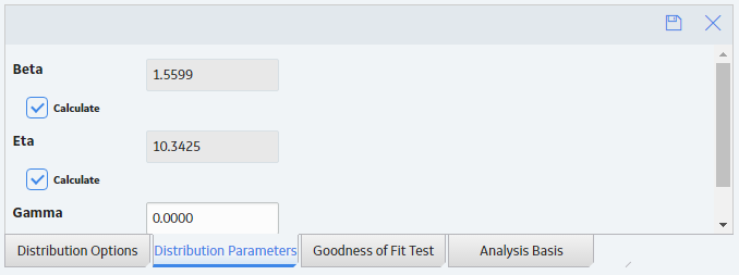
A Weibull Distribution describes the type of failure mode experienced by the population (infant mortality, early wear out, random failures, rapid wear-out). Estimates are given for Beta (shape factor) and Eta (scale). MTBF (Mean Time Between Failures) is based on characteristic life curve, not straight arithmetic average.

A Weibull Distribution uses the following parameters:

Beta: Beta, also called the shape factor, controls the type of failure of the element (infant mortality, wear-out, or random).
Eta: Eta is the scale factor, representing the time when 63.2 % of the total population is failed.
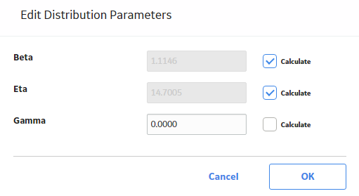
Gamma: Gamma is the location parameter that allows offsetting the Weibull distribution on time. The Gamma parameter should be used if the datapoints on the Weibull plot do not fall on a straight line.

If the value of Beta is greater than one (1), you can perform Preventative Maintenance (PM) Optimizations. A Gamma different from a value zero (0) means that the distribution is shifted to fit the datapoints more closely.

Note: This is an advanced feature and should be used in the proper context and with a good understanding of how to apply a three-parameter Weibull distribution.

Weibull Analysis Information

You can use the following information to compare the results of individual Weibull analyses. The following results are for good populations of equipment.


Beta Values Weibull Shape Factor
Components	Low	Typical	High	Low (days)	Typical (days)	High (days)
Ball bearing	0.7	1.3	3.5	583	1667	10417
Roller bearings	0.7	1.3	3.5	375	2083	5208
Sleeve bearing	0.7	1	3	417	2083	5958
Belts drive	0.5	1.2	2.8	375	1250	3792
Bellows hydraulic	0.5	1.3	3	583	2083	4167
Bolts	0.5	3	10	5208	12500	4166667
Clutches friction	0.5	1.4	3	2792	4167	20833
Clutches magnetic	0.8	1	1.6	4167	6250	13875
Couplings	0.8	2	6	1042	3125	13875
Couplings gear	0.8	2.5	4	1042	3125	52083
Cylinders hydraulic	1	2	3.8	375000	37500	8333333
Diaphragm metal	0.5	3	6	2083	2708	20833
Diaphragm rubber	0.5	1.1	1.4	2083	2500	12500
Gaskets hydraulics	0.5	1.1	1.4	29167	3125	137500
Filter oil	0.5	1.1	1.4	833	1042	5208
Gears	0.5	2	6	1375	3125	20833
Impellers pumps	0.5	2.5	6	5208	6250	58333
Joints mechanical	0.5	1.2	6	58333	6250	416667
Knife edges fulcrum	0.5	1	6	70833	83333	695833
Liner recip. comp. cyl.	0.5	1.8	3	833	2083	12500
Nuts	0.5	1.1	1.4	583	2083	20833
"O"-rings elastomeric	0.5	1.1	1.4	208	833	1375
Packings recip. comp. rod	0.5	1.1	1.4	208	833	1375
Pins	0.5	1.4	5	708	2083	7083
Pivots	0.5	1.4	5	12500	16667	58333
Pistons engines	0.5	1.4	3	833	3125	7083
Pumps lubricators	0.5	1.1	1.4	542	2083	5208
Seals mechanical	0.8	1.4	4	125	1042	2083
Shafts cent. pumps	0.8	1.2	3	2083	2083	12500
Springs	0.5	1.1	3	583	1042	208333
Vibration mounts	0.5	1.1	2.2	708	2083	8333
Wear rings cent. pumps	0.5	1.1	4	417	2083	3750
Valves recip comp.	0.5	1.4	4	125	1667	3333
Equipment Assemblies	Low	Typical	High	Low (days)	Typical (days)	High (days)
Circuit breakers	0.5	1.5	3	2792	4167	58333
Compressors centrifugal	0.5	1.9	3	833	2500	5000
Compressor blades	0.5	2.5	3	16667	33333	62500
Compressor vanes	0.5	3	4	20833	41667	83333
Diaphgram couplings	0.5	2	4	5208	12500	25000
Gas turb. comp. blades/vanes	1.2	2.5	6.6	417	10417	12500
Gas turb. blades/vanes	0.9	1.6	2.7	417	5208	6667
Motors AC	0.5	1.2	3	42	4167	8333
Motors DC	0.5	1.2	3	4	2083	4167
Pumps centrifugal	0.5	1.2	3	42	1458	5208
Steam turbines	0.5	1.7	3	458	2708	7083
Steam turbine blades	0.5	2.5	3	16667	33333	62500
Steam turbine vanes	0.5	3	3	20833	37500	75000
Transformers	0.5	1.1	3	583	8333	591667
Instrumentation	Low	Typical	High	Low (days)	Typical (days)	High (days)
Controllers pneumatic	0.5	1.1	2	42	1042	41667
Controllers solid state	0.5	0.7	1.1	833	4167	8333
Control valves	0.5	1	2	583	4167	13875
Motorized valves	0.5	1.1	3	708	1042	41667
Solenoid valves	0.5	1.1	3	2083	3125	41667
Transducers	0.5	1	3	458	833	3750
Transmitters	0.5	1	2	4167	6250	45833
Temperature indicators	0.5	1	2	5833	6250	137500
Pressure indicators	0.5	1.2	3	4583	5208	137500
Flow instrumentation	0.5	1	3	4167	5208	416667
Level instrumentation	0.5	1	3	583	1042	20833
Electro-mechanical parts	0.5	1	3	542	1042	41667
Static Equipment	Low	Typical	High	Low (days)	Typical (days)	High (days)
Boilers condensers	0.5	1.2	3	458	2083	137500
Pressure vessels	0.5	1.5	6	52083	83333	1375000
Filters strainers	0.5	1	3	208333	208333	8333333
Check valves	0.5	1	3	4167	4167	52083
Relief valves	0.5	1	3	4167	4167	41667
Service Liquids	Low	Typical	High	Low (days)	Typical (days)	High (days)
Coolants	0.5	1.1	2	458	625	1375
Lubricants screw compr.	0.5	1.1	3	458	625	1667
Lube oils mineral	0.5	1.1	3	125	417	1042
Lube oils synthetic	0.5	1.1	3	1375	2083	10417
Greases	0.5	1.1	3	292	417	1375

Weibull Results Interpretation

GE Digital APM Reliability shows the failure pattern of a single piece of equipment or groups of similar equipment using Weibull analysis methods. This helps you determine the appropriate repair strategy to improve reliability.

Is the Probability Plot a good fit?

Follow these steps to determine whether or not the plot is a good fit:

Identify Beta (slope) and its associated failure pattern.
Compare Eta (characteristic life) to standard values.
Check goodness of fit, compare with Weibull database.
Make a decision about the nature of the failure and its prevention.

The following chart demonstrates how to interpret the Weibull analysis data using the Beta parameter, Eta parameter, and typical failure mode to determine a failure cause.


Weibull Results			Interpretation
Beta	Eta	Typical Failure Mode	Failure Cause
Greater than 4	Low compared with standard values for failed parts (less than 20%)	Old age, rapid wear out (systematic, regular)	Poor machine design
Greater than 4	Low compared with standard values for failed parts (less than 20%)	Old age, rapid wear out (systematic, regular)	Poor material selection
Between 1 and 4	Low compared with standard values for failed parts (less than 20%)	Early wear out	Poor system design
Between 1 and 4	Low	Early wear out	Construction problem
Less than 1	Low	Infant Mortality	Inadequate maintenance procedure
Between 1 and 4	Between 1 and 4	Less than manufacturer recommended PM cycle	Inadequate PM schedule
Around 1	Much less than	Random failures with definable causes	Inadequate operating procedure

Goodness of Fit (GOF) Tests for a Weibull Distribution

A Goodness of Fit test is a statistical test that determines whether the analysis data follows the distribution model.

If the data passes the Goodness of Fit test, it means that it follows the model pattern closely enough that predictions can be made based on that model.
If the data fails the Goodness of Fit test, it means that the data does not follow the model closely enough to confidently make predictions and that the data does not appear to follow a specific pattern.

Weibull results are valid if Goodness of Fit (GOF) tests are satisfied. Goodness of Fit tests for a Weibull distribution include the following types:

R-Squared Linear regression (least squares): An R-Squared test statistic greater than 0.9 is considered a good fit for linear regression.
Kolmogorov-Smirnov: The GE Digital APM system uses confidence level and P-Value to determine if the data is considered a good fit. If the P-Value is greater than 1 minus the confidence level, the test passes.

Note: The R-Squared test statistic is calculated only for reference. The GE Digital APM system uses the Kolmogorov-Smirnov test as the Goodness of Fit test.

About Exponential Distribution

An Exponential Distribution is a mathematical distribution that describes a purely random process. It is a single parameter distribution where the mean value describes MTBF (Mean Time Between Failures). It is simulated by the Weibull distribution for value of Beta = 1. When applied to failure data, the Exponential distribution exhibits a constant failure rate, independent of time in service. The Exponential Distribution is often used in reliability modeling, when the failure rate is known but the failure pattern is not.

An Exponential Distribution uses the following parameter:

MTBF: Mean time between failures calculated for the analysis.

About Lognormal Distribution

In Lognormal Distributions of failure data, two parameters are calculated: Mu and Sigma. These do not represent mean and standard deviation, but they are used to calculate MTBF. In Lognormal analysis, the median (antilog of mu) is often used as the MTBF. The standard deviation factor (antilog of sigma) gives the degree of variance in the data.

A Lognormal Distribution uses the following parameters:

Mu: The logarithmic average for the Distribution function.
Sigma: The scatter.
Gamma: A location parameter.

About Triangular Distribution

Triangular Distribution is typically used as a subjective description of a population for which there is only limited sample data, and especially in cases where the relationship between variables is known, but data is scarce (possibly because of the high cost of collection). It is based on a knowledge of the minimum (a) and maximum (b) and an inspired guess as to the modal value (c).

A Triangular Distribution is a continuous Probability Distribution with:

Lower limit a
Upper limit b
Mode c

…where a < b and a ≤ c ≤ b.

About Gumbel Distribution

The Gumbel Distribution is a continuous probability distribution. Gumbel distributions are a family of distributions of the same general form. These distributions differ in their location and scale parameters: the mean of the distribution defines its location, and the standard deviation, or variability, defines the scale.

The Gumbel Distribution is a probability distribution of extreme values.

In probability theory and statistics, the Gumbel distribution is used to model the distribution of the maximum (or the minimum) of a number of samples of various distributions.

About Generalized Extreme Value Distribution

In probability theory and statistics, the Generalized Extreme Value (GEV) Distribution is a family of continuous probability distributions developed within extreme value theory.

By the Extreme Value Theorem, the GEV Distribution is the only possible limit distribution of properly normalized maxima of a sequence of independent and identically distributed random variables.

Change the Distribution Parameters in a Probability Distribution Analysis

About this task

This topic describes how to modify the values of the distribution parameters in a Probability Distribution Analysis.

You can change the distribution parameters from the Analysis Summary workspace or from any of the plot tabs in the left pane.

Procedure

Access a Probability Distribution Analysis for which you want to modify the Distribution Parameters.
If you want to modify the values of the Distribution Parameters from the Analysis Summary workspace:
1. In the bottom section, select Distribution Parameters, and then select .
  
  The Calculate check boxes appear below each of the parameters.
2. Clear the Calculate check box next to the parameter(s) whose value you want to modify.
  
  The parameter field(s) are enabled.
3. Enter the desired value for the parameter.
4. Select .
  Note: If you reselect the Calculate check box after manually entering data, the manually entered data for the parameter will not be retained. If you decide not to use the parameters you entered, select , and the previous selection will be used in the calculations.
  
  The system recalculates the analysis based on the selected distribution parameter.
-or-

If you want to modify the values of the distribution parameters from one of the plot tabs (e.g., Probability Plot tab):
1. In the left pane, select the Probability Plot tab.
  
  The Probability Plot appears in the workspace.
  
  Note: You can also change distribution parameter via the PDF Plot or CDF Plot tabs.
2. In the upper-right corner of the workspace, select Distribution Options, and then select Distribution Parameters.
  The Edit Distribution Parameters window appears.
3. Clear the Calculate check box next to the parameter(s) whose value you want to modify.
  The parameter field(s) are enabled.
4. Enter the desired value for the parameter, and then select OK.
  Note: If you reselect the Calculate check box after manually entering data, the manually entered data for the parameter will not be retained. If you decide not to use the parameters you entered, select Cancel, and the previous selection will be used in the calculations.
  The system recalculates the analysis based on the selected distribution parameter.

Change the Fit Method of a Probability Distribution Analysis

About this task

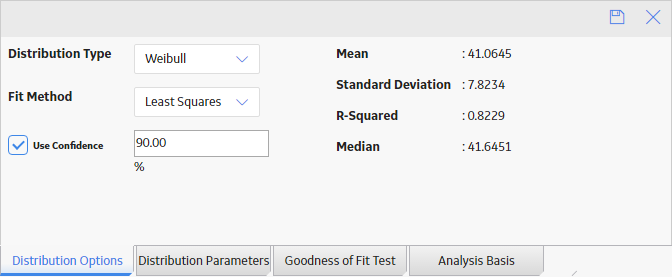
The Kolmogorov-Smirnov test is a Goodness of Fit (GOF) test applied to a Probability Distribution Analysis to determine how well the data fits the analytical curve. When you create an analysis, the fit method is set to Least Squares by default.

After the analysis is created, you can modify the fit method to one of the following:

Least Squares: A curve-fitting estimation method that relies on linear regression techniques to estimate the parameters for the distribution.
Maximum Likelihood Estimators: A curve-fitting estimation method that maximizes the likelihood function for a given population. This method includes a survivor function that estimates changes in reliability as the piece of equipment or location survives beyond a certain age.

You can change the fit method from the Analysis Summary workspace or from any of the plot tabs in the left pane.

Procedure

Access a Probability Distribution Analysis for which you want to modify the Fit Method.
If you want to change the Fit Method from the Analysis Summary workspace:
1. In the bottom section, select Distribution Options, and then select .
  The Fit Method field is enabled.
2. In the Fit Method box, select the desired Fit Method, and then select .
  The analysis is recalculated based on the selected Fit Method.
-or-

If you want to change the Fit Method from one of the plot tabs (e.g., Probability Plot tab):
1. In the left pane, select the Probability Plot tab.
  The Probability Plot appears in the workspace.
  
  Note: You can also change the Fit Method via the PDF Plot or CDF Plot tabs.
2. In the upper-right corner of the workspace, select Distribution Options, and then select Fit Method.
  The Edit Fit Method window appears.
3. Select the desired Fit Method, and then select OK.
  The analysis is recalculated based on the selected Fit Method.

Modify the Confidence Level for a Probability Distribution Analysis

About this task

The Confidence Level specifies how the optimistic and realistic scenarios will be selected in a Monte Carlo Simulation for TTR Distributions in an analysis. The Confidence Level indicates whether the distribution is within the confidence limits or not. The default Confidence Level for an analysis is 90 percent.

You can modify the Confidence Level from the Analysis Summary workspace or from any of the plot tabs in the left pane.

Procedure

Access a Probability Distribution Analysis for which you want to modify the Confidence Level.
If you want to change the Confidence Level from the Analysis Summary workspace:
1. In the bottom section, select Distribution Options, and then select .
  The Confidence Level field is enabled.
  
  Note: If the Confidence Level field is disabled, select the Use Confidence check box to activate the confidence level and enable the Confidence Level field.
2. In the Confidence Level box, select the desired Confidence Level, and then select .
  The GE Digital APM system displays the confidence intervals for the analysis based on the percentage you entered in the Confidence Level field.
-or-

If you want to change the Confidence Level from one of the plot tabs (e.g., Probability Plot tab):
1. In the left pane, select the Probability Plot tab.
  The Probability Plot appears in the workspace.
  
  Note: You can also change the Confidence Level via the PDF Plot or CDF Plot tabs.
2. In the upper-right corner of the workspace, select Distribution Options, and then select Fit Method.
  The Select Confidence Level window appears.
3. Select the desired Confidence Level, and then select OK.
  The GE Digital APM system displays the confidence intervals for the analysis based on the percentage you entered in the Confidence Level field.

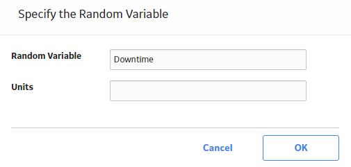
Modify the Random Variable and Specify Units for a Probability Distribution Analysis

Procedure

Access a Probability Distribution Analysis for which you want to modify the value of Random Variable and specify units.
In the left pane, select the Probability Plot tab.

The Probability Plot appears in the workspace.

Note: You can also modify the value of Random Variable and specify units via the PDF Plot or CDF Plot tabs.
In the upper-right corner of the workspace, select Analysis Task, and then select Change Units.

The Specify the Random Variable window appears.
In the Random Variable box, enter the name of the Random Variable.
In the Units box, enter the corresponding units, and then select OK.

The analysis is recalculated using the new Random Variable.

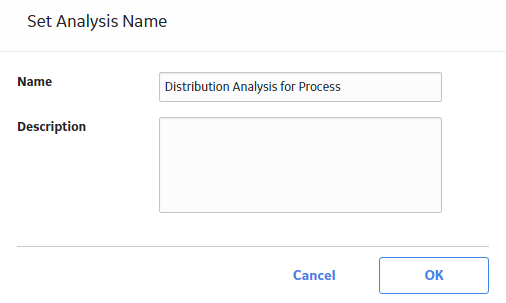
Rename a Probability Distribution Analysis

Procedure

Access a Probability Distribution Analysis whose name you want to change.
In the left pane, select the Probability Plot tab.

The Probability Plot appears in the workspace.

Note: You can also modify the value of Random Variable and specify units via the PDF Plot or CDF Plot tabs.
In the upper-right corner of the workspace, select Analysis Task, and then select Rename.

The Set Analysis Name window appears.
In the Name box, enter a new name for the analysis.
In the Description box, enter a new description for the analysis, and then select OK.

The analysis name is updated in all the appropriate sections on the Probability Distribution page. In addition, the Description field in any appropriate sections will reflect any changes.

Access the Source Data for a Probability Distribution Analysis

Procedure

Access a Probability Distribution Analysis for which you want to view the data.
In the left pane, select Probability Plot.

The Probability Plot appears in the workspace.

Note: You can also view the data via the PDF Plot or CDF Plot tabs.
In the upper-right corner of the workspace, select Analysis Data, and then select Go To Source.
The fields on the page that appears display the analysis data associated with the selected Probability Distribution Analysis correspond to values that were used to create the analysis.
- For an analysis based on a query, the information returned by the query appears.
- For an analysis based on a dataset, the information stored in the dataset appears.
- For an analysis based on manually-entered data, you will receive the following error message:
  
  There is no source data to view since the analysis is based on manually entered data.
  
  To view data for an analysis based on manually-entered data, you can access the Probability Distribution Data window.

Modify Data in a Probability Distribution Analysis

Procedure

Access a Probability Distribution Analysis for which you want to modify the data.
In the left pane, select Probability Plot.

The Probability Plot appears in the workspace.

Note: You can also modify the data via the PDF Plot or CDF Plot tabs.
In the upper-right corner of the workspace, select Analysis Data, and then select View Data.

The Probability Data Editor window appears, displaying the data associated with the selected Probability Distribution Analysis.
As needed, modify the data in any enabled field, and then select OK.

The analysis is updated to reflect any changes that you made.

Results

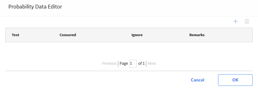
For an analysis that is based on manually entered data, the changes that you make via the Probability Distribution Data window will be saved for the analysis.
For an analysis that is based on a query or a dataset:
- The query or dataset will not be modified with the updated data. Additionally, any record returned by the query will not be updated with your changes. The changes will be saved to the analysis only.
- After you modify the data and save the analysis, the modified data will appear each time you open the analysis. If you want to revert to the original data, you can reload the original data to the analysis. In addition, if a query or dataset has changed in the database, you can reload the data in order for your analysis to contain those changes.

Reload Analysis Data in a Probability Distribution Analysis

About this task

When you create and save an analysis that is based on a query or dataset, the GE Digital APM system takes a snapshot of the data that exists at the time of creation and saves it along with the analysis. When you open an existing analysis, the GE Digital APM system loads the data that was last saved with the analysis. This means that any changes to the underlying query or dataset will not be reflected automatically when you open an existing analysis.

Note: If the query or dataset has been deleted or renamed, when you try to open an associated analysis, an error message will be displayed and the data will not be refreshed.

If you want to refresh an analysis based upon changes to the underlying query or dataset or to load new data that has been added since the analysis was last saved (e.g., the analysis is based on a query that retrieves failures for a piece of equipment or location, and a new failure record has been added to the database), you will need to reload the analysis manually after opening it. When you reload the data, any manual changes made to the analysis data set will be deleted.

Note: Reloading analysis data resets the analysis period only if it is based on the analysis data. Start Dates and End Dates that have been set explicitly will not be overwritten.

Procedure

Access a Probability Distribution Analysis for which you want to reload the data.
In the left pane, select Probability Plot.

The Probability Plot appears in the workspace.

Note: You can also reload the data via the PDF Plot or CDF Plot tabs.
In the upper-right corner of the workspace, select the Analysis Data list, and then select Reload Data.

A confirmation message appears, asking you to confirm that you want to overwrite the current data with the data stored in the database.

Note:
For an analysis based on manually-entered data, you will receive the following error message:

There is no source data to reload since the analysis is based on manually entered data.
Select Yes.

The analysis is updated to reflect the data currently stored in the query or dataset.

Note: If you are reloading analysis data that is based on a query and an index out of range error message appears, there is an error in the query. You should modify the query or recreate the analysis in order to reload the correct data.

Censor Data in a Probability Distribution Analysis

Procedure

Access the Probability Distribution Analysis, which contains the plot in which you want to censor a datapoint.
In the left pane, select the plot in which you want to censor a datapoint.
In the plot, select the desired datapoint.

The Probability Data Editor window appears.
In the Censored column, select the check box for the desired datapoint.

The selected datapoint is censored or ignored in the Probability Distribution Analysis.

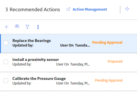
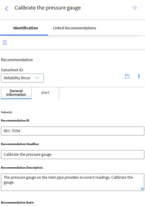
Access a Recommendation

Procedure

Access the analysis for which you want to create a recommendation.
In the right corner of the workspace, select the .
The Recommendations pane appears, displaying a list of recommendations associated with the selected analysis.
Select the row containing the recommendation that you want to view.
The Reliability Recommendation datasheet appears, displaying the General Information and Alert tabs.

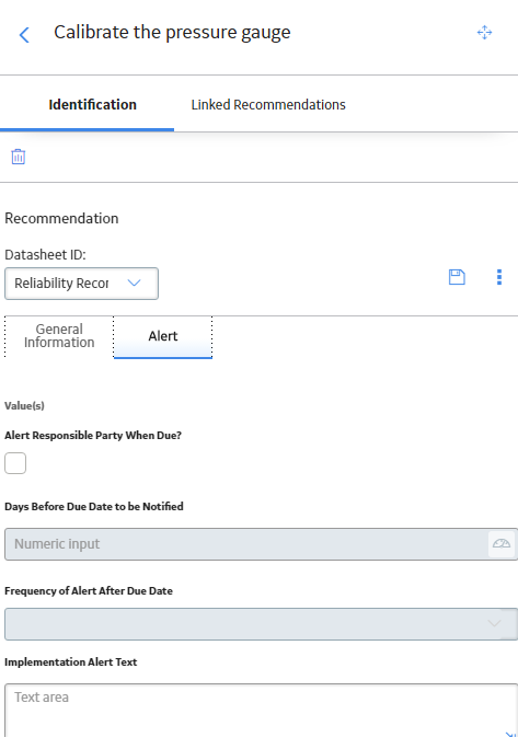
Create a Recommendation Alert for an Analysis

Procedure

Access the analysis from which you want to generate an alert.

The Reliability Recommendation datasheet appears.
Select the Alert tab.
The Alert datasheet appears.
As needed, enter values in the available fields, and then select .
The Alert is saved.

Delete a Probability Distribution Analysis

Procedure

Access the RA Overview page.
Select the Probability Distribution tab.

A list of Probability Distribution Analyses available in the database appears.
Select the row containing the Probability Distribution Analysis that you want to delete, and then select .

The Delete Probability Distribution Analysis dialog box appears, asking you to confirm that you want to delete the selected analysis.
Select Yes.

The selected analysis is deleted.

Access Probability Distribution Report

Procedure

Access the Probability Distribution Analysis whose report you want to access.
In the upper-right corner of any workspace within the selected Probability Distribution Analysis, select Report.
The Probability Distribution Analysis report appears in a new tab.

By default, the report contains the following sections:
- Analysis Plots
- Analysis Summary
- Statistical Distribution Information
- Distribution Data

About Probability Distribution Report

The baseline GE Digital APM database includes the Probability Distribution report, which you can use to view a summary of the results of a Probability Distribution Analysis.

The Probability Distribution report is built from the following Catalog items:

The subreport, SubReportProbDist, which is stored in the Catalog folder \\Public\Meridium\Modules\Reliability Manager\Reports.
The supporting queries that supply data in the main report and subreport, which are stored in the Catalog folder \\Public\Meridium\Modules\Reliability Manager\Reports. The following supporting queries are available:
- ProbabilityDistributionQuery
- Weibull Distribution Query
- Lognormal Distribution Query
- Normal Distribution Query
- Exponential Distribution Query

Throughout this documentation, we refer to the main report, the subreport, and the supporting queries collectively as the Probability Distribution report.

The Probability Distribution report contains a prompt on the ENTY KEY and Distribution Type fields in the Distribution family. When you run the Probability Distribution report via the Probability Distribution module, the ENTY KEY and Distribution Type of the Distribution record associated with the current analysis is passed automatically to the prompt, and the results for the current Probability Distribution Analysis are displayed. If you run the main report or any of the queries in the preceding list directly from the Catalog, however, you will need to supply the ENTY KEY and Distribution Type of a Distribution record manually to retrieve results. The subreport (i.e., Catalog item SubReportProbDist) cannot be run directly from the Catalog.

Analysis Summary Section

The Analysis Summary section of the Probability Distribution report displays information that is stored in a Distribution record. Distribution records are categorized into one of four Distribution subfamilies: Exponential, Lognormal, Normal, or Weibull.

The following table lists each item in the Analysis Summary section and the corresponding Distribution record field whose data is displayed in the report.


Report Item	Distribution record
Analysis Name	Analysis ID
Analysis Description	Short Description
Random Variable	Random Variable Field
Units	Units
Last Modified	LAST UPDT DT
Modified By	LAST UPBY SEUS KEY Note: The name of the Security User associated with this value is displayed in the report.

Statistical Distribution Information Section

The Statistical Distribution Information section of the Probability Distribution report displays information that is stored in the Distribution record (i.e., Exponential, Lognormal, Normal, or Weibull record).

The following subsections are displayed within the Statistical Distribution Information section:

The Distribution Type subsection displays information that is stored in the Distribution record. Throughout the documentation, we will refer to this subsection as the Distribution subsection.

The following table lists each item in the Distribution subsection and the corresponding Distribution record field whose data is displayed in the report.


Report Item	Distribution Field
Distribution Type	Distribution Type
Fit Method	Fit Method
Use Confidence	Use Confidence
Confidence Level	Confidence Level
Mean	Mean
Standard Deviation	Standard Deviation
Median	Median
R2	R-Squared

The Parameters subsection contains information stored in the Distribution record. The type of information that appears in the Parameters subsection depends on the distribution type (i.e., Weibull, Lognormal, Exponential, or Normal).

The following table lists each item in the Parameters subsection for a Weibull record whose data is displayed in the report. One row is displayed for each of the following field captions: Beta, Eta, and Gamma.


Report Item	Weibull Field
Beta
Value	Beta
Low	Beta Low
High	Beta High
Calculated	Beta Fixed
Eta
Value	Eta
Low	Eta Low
High	Eta High
Calculated	Eta Fixed
Gamma
Value	Gamma
Low	Gamma Low
High	Gamma High
Calculated	Gamma Fixed

The following table lists each item in the Parameters subsection for a Lognormal record whose data is displayed in the report. For a Lognormal record, one row is displayed for each of the following field captions: Mu, Sigma, and Gamma.


Report Item	Lognormal Field
Mu
Value	Mu
Low	Mu Low
High	Mu High
Calculated	Mu Fixed
Sigma
Value	Sigma
Low	Sigma Low
High	Sigma High
Calculated	Sigma Fixed
Gamma
Value	Gamma
Low	Gamma Low
High	Gamma High
Calculated	Gamma Fixed

The following table lists each item in the Parameters subsection for an Exponential record whose data is displayed in the report. For an Exponential record, one row is displayed for the field caption MTBF.


Report Item	Exponential Field
MTBF
Value	MTBF
Low	MTBF Low
High	MTBF High
Calculated	MTBF Fixed

The following table lists each item in the Parameters subsection for a Normal record whose data is displayed in the report. For a Normal record, one row is displayed for each of the following field captions: Mean, Standard Deviation.


Report Item	Normal Field
Mean
Value	Mean
Low	Mean Low
High	Mean High
Calculated	Mean Fixed
Standard Deviation
Value	Standard Deviation
Low	Standard Deviation Low
High	Standard Deviation High
Calculated	Standard Deviation Fixed

The Goodness of Fit Test subsection displays information from the Distribution record.

The Kolmogorov-Smirnov test is the only test used to measure goodness of fit, so the Name column in the report is populated with the value Kolmogorov-Smirnov Test.

The following table lists each remaining item in the Goodness of Fit Test subsection and the Distribution record field whose data is displayed in the report.


Report Item	Weibull Field
Statistic	GOF Statistic
P-Value	GOF P-Value
Passed	Passed

Distribution Data Section

The Distribution Data section of the Probability Distribution report displays information that is stored in the Data field in the Distribution record.

The following values are displayed in the Distribution Data section, and they are stored in the Data field in the Reliability Distribution record:

X (i.e., the Random Variable)
Censored
Ignored
Remarks

Plots Section

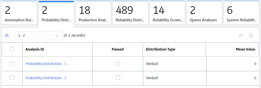
The Plots section of the Probability Distribution report displays the plots that are displayed on the Analysis Summary workspace or accessed via the Plots tabs in the left pane on the Probability Distribution page.

The Plots section displays the following graphs: