Confidence Level and P Value
About Confidence Level and P-Value
In a Distribution Analysis, the Confidence Level and the P-Value are used to determine whether the data passes the Goodness of Fit test.
The Confidence Level indicates the percentage of uncertainty of the Goodness of Fit method. This percentage is usually determined by experience or an industry standard and limits how closely the data must fit the model in order for it to pass the Goodness of Fit test. The higher the Confidence Level, the farther apart your confidence bounds will be, and the easier it will be for your data to pass the Goodness of Fit test. The lower the Confidence Level and the closer together the bounds are, the harder it will be for your data to pass the Goodness of Fit test. If the data does pass, however, the data will be a very close fit to the model.
About Data Censoring in a Reliability Distribution Analysis
Reliability Distribution Analysis supports the functionality of censoring, which accounts for the period of time from the last failure date to the analysis end date. You can censor or ignore datapoints in a Reliability Distribution Analysis to estimate the probability of when a failure might occur. Censoring is based on failure modes.
Details
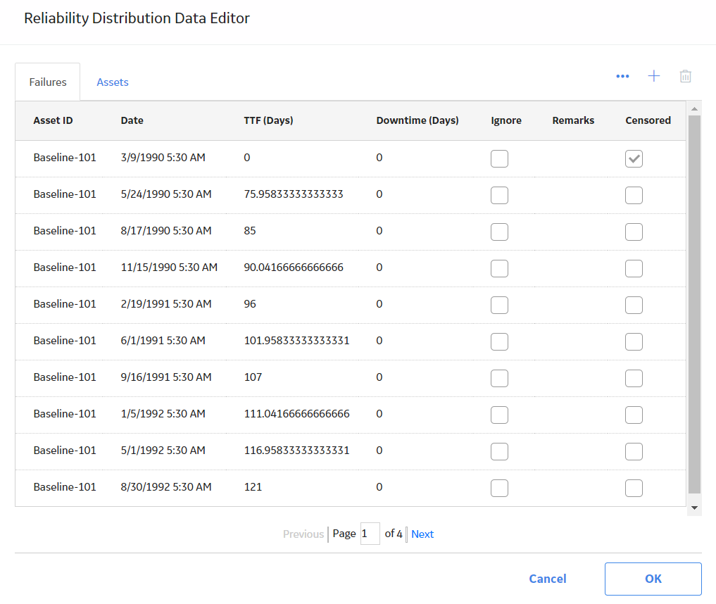
Censoring a datapoint means that the datapoint is excluded as a failure but included in the operating time of the piece of equipment. If you select the Censored check box, the data in the selected row is excluded. When you create a Reliability Distribution Analysis using a query or dataset as the data source, the GE Digital APM system automatically censors time values from the beginning of the Analysis Period to the first event and the time value from the last event to the end of the analysis. After the calculations for the analysis have been performed, each time that the query or dataset is refreshed, the censoring settings will be reset using the default criteria. Therefore, if you select a check box and refresh the data, the check boxes will no longer be selected.
Regardless of the data source you use, you can censor any failure data. Consider the following:
- For Maximum Likelihood Estimators (MLE), the maximum number of censored datapoints is one (1) less than the total number of datapoints.
- For Least Squares estimation, the maximum number of censored datapoints is two (2) less than the total number of datapoints.
Pump Failure
Assume that you want to determine the reasons due to which a pump failed.
A pump might have failed due to multiple reasons, such as rusted part, motor overheating, insufficient power supply, or power outage. Each of these reasons will have its own specific failure rate and probability density function. To determine the failure rate of "motor overheating", you must censor all other failure modes from the analysis.
Further, motor overheating might be caused due to multiple reasons, such as improper operation, improper application, and improper maintenance. The censoring feature allows you to separate the failure modes, and determine which is the dominant failure mode. Based on this information, you can decide what is needed to improve the motor performance.
Auto-Censoring
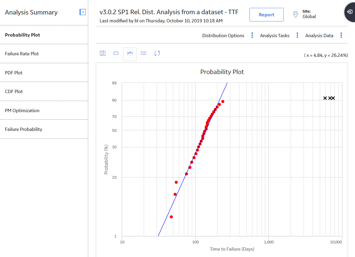
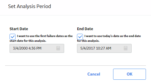
When you first create a Reliability Distribution Analysis, an automatically censored datapoint for each defined asset will appear on the plot. Each automatically censored datapoint represents the analysis End Date (specified on the Set Analysis Period window) for each defined asset.
GE Digital APM can:
- Censor failures automatically when it cannot calculate the time between events. For example, failure on a specific asset where the analysis does not contain a start date.
- Alert you that a datapoint is suspect. For example, in a Time to Failure type of distribution, an alert will be generated when the start date of an event overlaps the end date of a different event for the same asset. For this asset, suspect data is displayed in the Analysis Summary workspace.
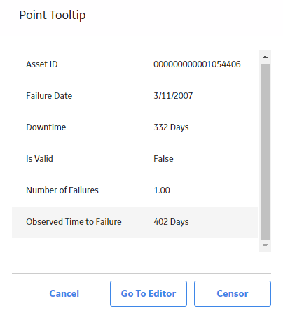
For a Reliability Distribution Analysis, when you pause on an automatically censored datapoint, the following information appears:
- Auto-Censored
- Name: Specified on the Assets tab of the Reliability Distribution Data Editor window.
- Installation Date: Specified in the Assets section of the Reliability Distribution Data Editor window.
- TTF value: Represents the time between the last failure date and the analysis End Date.
Modify the Confidence Level for a Reliability Distribution Analysis
About This Task
The Confidence Level specifies how the optimistic and realistic scenarios will be selected in a Monte Carlo Simulation for TTR Distributions in an analysis. The Confidence Level indicates whether the distribution is within the confidence limits or not. The default Confidence Level for an analysis is 90 percent.
You can modify the Confidence Level in the Analysis Summary workspace or after selecting any of the plot tabs in the left pane.
Procedure
Change the Failure Type in a Reliability Distribution Analysis
About This Task
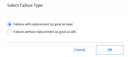
You can change the failure type in the any of the plots selectable via the plot tabs in the left pane (i.e., Probability Plot tab, Failure Rate Plot tab, PDF Plot tab, CDF Plot tab, and Failure Probability tab). These instructions describe how to change the failure type in the Probability Plot
Procedure
Modify the Analysis Period
Procedure
Choose the Time Units for an Analysis
About This Task
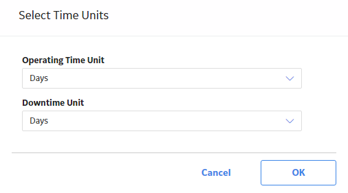
The time units are used for expressing time values for calculations performed within an analysis. For example, a calculation may indicate the amount of time that lapsed between a failure event and the end date of the analysis period. This value would be expressed in the Time Units for the analysis.
Your Time Units selection will depend on what type of data you are using and what type of analysis you are performing. For example, in an analysis that shows the distribution of failures for a number of pieces of equipment or locations over many years, years might be an appropriate unit of time. For an analysis designed to evaluate failures for a single piece of equipment or location within a very specific time period, a smaller unit of time would be appropriate. For this reason, you can choose the Time Units that are most appropriate for a given analysis.
Procedure
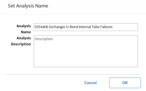
Rename a Reliability Distribution Analysis
Procedure
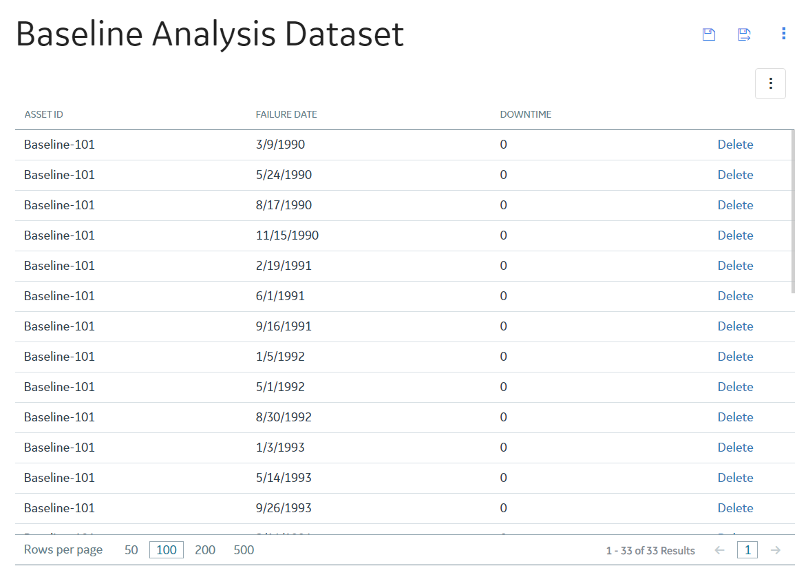
Access the Source Data for a Reliability Distribution Analysis
About This Task
You can access the source data only if the analysis is based on a query or a dataset.
Procedure
Modify the Data in a Reliability Distribution Analysis
Procedure
Results
- For an analysis that is based on manually entered data, the changes that you make via the Reliability Distribution Data window will be saved for the analysis.
- For an analysis that is based on a query or a dataset:
- The query or dataset will not be modified with the updated data. Additionally, any record returned by the query will not be updated with your changes. The changes will be saved to the analysis only.
- After you modify the data and save the analysis, the modified data will appear each time you open the analysis. If you want to revert to the original data, you can reload the original data to the analysis. In addition, if a query or dataset has changed in the database, you can reload the original data to the analysis in order for your analysis to contain those changes.
Reload Analysis Data in a Reliability Distribution Analysis
About This Task
When you create and save an analysis that is based on a query or dataset, the GE Digital APM system takes a snapshot of the data that exists at the time of creation and saves it along with the analysis. When you open an existing analysis, the GE Digital APM system loads the data that was last saved with the analysis. This means that any changes to the underlying query or dataset will not be reflected automatically when you open an existing analysis.
If you want to refresh an analysis based on changes to the underlying query or dataset or to load new data that has been added since the analysis was last saved (e.g., the analysis is based on a query that retrieves failures for a piece of equipment or location, and a new failure record has been added to the database), you will need to reload the analysis manually after opening it. When you reload the data, any manual changes made to the analysis data set will be deleted.
Procedure
Censor Data in a Reliability Distribution Analysis
Procedure
Perform a Preventive Maintenance Optimization
About This Task
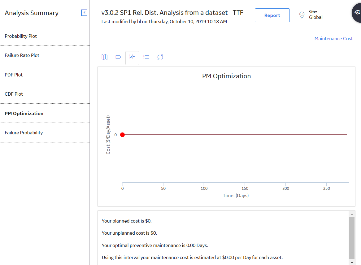
A PM Optimization involves several steps. Based on the MTBF and the calculation of the ratios, the system estimates the optimum time interval to maintain equipment.
PM Optimization is available only if Failures With Replacements was selected as the failure type via the Reliability Distribution Builder
or Failure Type window.PM Optimization is not available when Beta is less than or equal to one (Beta <= 1).
Procedure
About Preventive Maintenance Optimization
Preventative Maintenance (PM) Optimization uses the results of a Reliability Distribution Analysis to measure the optimum time to perform a Planned (Restorative) Maintenance (PM) procedure on a piece of equipment. PM optimization does not calculate minor maintenance schedules but determines the optimal time to perform major repairs or replace a piece of equipment until there is a minimal amount of cost and risk. PM optimization is only valid for wear-out failure modes and will not give accurate results for a Weibull analysis where Beta is less than 1.
Details
A PM optimization is composed of the following steps:
- The calculation model is configured to acquire the necessary parameters, including Mean Time Between Failures (MTBF). MTBF is used to determine the probability that a piece of equipment will fail.
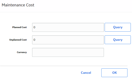
- The cost ratio is determined. This ratio is the cost of planned Preventative Maintenance (PM) events versus the cost of unplanned maintenance events. You can manually enter the cost or select an existing query as the source of the cost data.
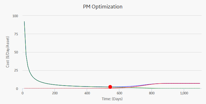
- Based on the MTBF and the calculation of the ratios, the GE Digital APM system estimates the optimum time (interval) to maintain equipment. The cost per piece of equipment based on the Optimized Preventative Maintenance Interval is also displayed.
- The GE Digital APM system creates optimization graphs, which gives the analyst the optimum time to conduct a repair or overhaul based upon the ratio of planned to unplanned repair costs. This ensures that repairs are conducted in a cost-effective manner, minimizing risk while maximizing time in service.
The limitation to using a PM optimization is it will always give a result for the statistical distribution on which it is based. This does not mean that it will always make sense to do a PM at the interval specified. In particular, design flaws that manifest themselves as poor reliability can more effectively be addressed through redesign rather than PM.
Access Reliability Distribution Analysis Report
Procedure
About Reliability Distribution Analysis Report
The baseline GE Digital APM database includes the Reliability Distribution Analysis report, which you can use to view a summary of the results of a Reliability Distribution Analysis.
The Reliability Distribution Analysis report is built from the following Catalog items:
- The main report, DistributionAnalysisReport, which is stored in the Catalog folder \\Public\Meridium\Modules\Reliability Manager\SSRS.
- The subreport, SubreportDistributionAnalysis, which is stored in the Catalog folder \\Public\Meridium\Modules\Reliability Manager\Reports.
- The subreport, assetSubreportDistribution, which is stored in the Catalog folder \\Public\Meridium\Modules\Reliability Manager\Reports.
- The supporting queries that supply data in the main report and subreports, which are stored in the Catalog folder \\Public\Meridium\Modules\Reliability Manager\Reports. The following supporting queries are available:
- ReliabilityDistributionQuery
- ReliabilityDistributionTTR
- ReliabilityExponentialTTF
- ReliabilityExponentialTTR
- ReliabilityLognormalTTF
- ReliabilityLognormalTTR
- ReliabilityNormalTTF
- ReliabilityNormalTTR
- ReliabilityWeibullTTF
- ReliabilityWeibullTTR
Throughout this documentation, we refer to the main report, the subreports, and the supporting queries collectively as the Reliability Distribution Analysis report.
Analysis Summary Section
The Analysis Summary section of the Reliability Distribution report displays information that is stored in the Reliability Distribution record and Distribution records that are linked to the Reliability Distribution record.
The following table lists each item in the Analysis Summary section and the corresponding Reliability Distribution or Distribution record field whose data is displayed in the report.
| Report Item | Record | Record Field |
|---|---|---|
| Analysis Name | Reliability Distribution | Analysis ID |
| Analysis Description | Reliability Distribution | Short Description |
| Analysis Start | Reliability Distribution | Analysis Start Date |
| Analysis End | Reliability Distribution | Analysis End Date |
| Number of Assets | Reliability Distribution | Assets |
| Number of Failures | Reliability Distribution | Number of Failures |
| Censored Failures | Reliability Distribution | Censored Failures |
| MTBF | Reliability Distribution | MTBF |
| MTTR | Reliability Distribution | MTTR |
| Use Confidence | Reliability Distribution | Use Confidence |
| Confidence Level | Distribution | Confidence Level |
| Last Modified | Reliability Distribution | LAST UPDT DT |
| Modified By | Reliability Distribution |
LAST UPBY SEUS KEY Note: The name of the Security User associated with this value is displayed in the report.
|
Statistical Distribution Information Section
The Statistical Distribution Information section of the Reliability Distribution report displays information that is stored in each Distribution record that is linked to the Reliability Distribution record. Each Distribution record is a member of one of four Distribution subfamilies in which records can exist: Exponential, Lognormal, Normal, or Weibull.
The following subsections are displayed for each Distribution record that is linked to the Reliability Distribution:
In the <Variable> Distribution subsection, <Variable> is the value that is stored in the Variable field in the Distribution record that is linked to the Reliability Distribution record. Throughout the documentation, we will refer to this subsection as the Distribution subsection.
The following table lists each item in the Distribution subsection and the corresponding Distribution record field whose data is displayed in the report.
| Report Item | Distribution Field |
|---|---|
| Distribution Type |
Distribution Type |
| Operating Time Units |
Units |
| Fit Method |
Fit Method |
| R2 | R-Squared |
| Mean | Mean |
| Standard Deviation | Standard Deviation |
| Median |
Median |
The Parameters subsection contains information stored in a Distribution record (i.e., Weibull, Lognormal, Exponential, or Normal record). The Weibull, Lognormal, Exponential, or Normal record is linked to the Reliability Distribution record. The items that appear in the Parameters subsection will be different, depending on the type of Distribution record.
The following table lists each item in the Parameters subsection for a Weibull record whose data is displayed in the report. For a Weibull record, one row is displayed for each of the following field captions: Beta, Eta, and Gamma.
| Report Item | Weibull Field |
|---|---|
| Beta | |
| Value |
Beta |
| Low |
Beta Low |
| High | Beta High |
| Calculated | Beta Fixed |
| Eta | |
| Value | Eta |
| Low | Eta Low |
| High |
Eta High |
| Calculated | Eta Fixed |
| Gamma | |
| Value | Gamma |
| Low | Gamma Low |
| High |
Gamma High |
| Calculated | Gamma Fixed |
The following table lists each item in the Parameters subsection for a Lognormal record whose data is displayed in the report. For a Lognormal record, one row is displayed for each of the following field captions: Mu, Sigma, and Gamma.
| Report Item | Lognormal Field |
|---|---|
| Mu | |
| Value |
Mu |
| Low |
Mu Low |
| High | Mu High |
| Calculated | Mu Fixed |
| Sigma | |
| Value | Sigma |
| Low | Sigma Low |
| High |
Sigma High |
| Calculated | Sigma Fixed |
| Gamma | |
| Value | Gamma |
| Low | Gamma Low |
| High |
Gamma High |
| Calculated | Gamma Fixed |
The following table lists each item in the Parameters subsection for an Exponential record whose data is displayed in the report. For an Exponential record, one row is displayed for the field caption MTBF.
| Report Item | Exponential Field |
|---|---|
| MTBF | |
| Value |
MTBF |
| Low |
MTBF Low |
| High | MTBF High |
| Calculated | MTBF Fixed |
The following table lists each item in the Parameters subsection for a Normal record whose data is displayed in the report. For a Normal record, one row is displayed for each of the following field captions: Mean, Standard Deviation.
| Report Item | Normal Field |
|---|---|
| Mean | |
| Value |
Mean |
| Low |
Mean Low |
| High | Mean High |
| Calculated | Mean Fixed |
| Standard Deviation | |
| Value | Standard Deviation |
| Low | Standard Deviation Low |
| High |
Standard Deviation High |
| Calculated | Standard Deviation Fixed |
The Goodness of Fit Test subsection displays information from the corresponding Distribution record.
The Kolmogorov-Smirnov test is the only test used to measure goodness of fit, so the Name column in the report is populated automatically with the value Kolmogorov-Smirnov test. The following table lists each remaining item in the Goodness of Fit Test subsection and the corresponding Distribution record field whose data is displayed in the report.
| Report Item | Distribution Field |
|---|---|
| Statistic |
GOF Statistic |
| P-Value |
GOF P-Value |
| Passed |
Passed |
Assets Section
The Assets section of the Reliability Distribution report displays information that is stored in the Failure Data field in the Reliability Distribution record.
The following values are displayed in the Assets section:
- Asset ID
- Installation Date
- Last Replacement
- Present Age
- Future Age
- Present Failure Probability
- Future Failure Probability
Functional Failures Section
The Functional Failures section of the Reliability Distribution report displays information that is stored in the Failure Data field in the Reliability Distribution record.
The following values are displayed in the Failure Data section:
- Asset ID
- Failure Date
- TTF
- Downtime
- Ignore
- Censored
- Remarks
Analysis Plots Section
The Analysis Plots section of the Reliability Distribution report displays the graphs that are displayed in the Time to Failure Distribution section or accessed via the left pane in the Analysis Summary workspace for the selected analysis.
The Plots section displays the following graphs:
 .
. .
.