Reliability Distribution Analyses

About Reliability Distribution Analysis

A Reliability Distribution Analysis allows you to describe the Time to Failure (TTF) as a statistical distribution, which is usually characterized by a specific pattern. The following distribution types are supported:

The Reliability Distribution Analysis characterizes how failures are distributed over the life of equipment. Analyzing the distribution of failures means examining a particular failure mode over one or multiple pieces of equipment. Generating a Distribution Analysis will help you find the answers to the following questions:

  • Do most of the equipment failures occur early on?
  • Does the equipment fail more at the end of its span of service?  
  • Are the failures fairly evenly distributed throughout the life of the equipment or randomly occurring?

In a Reliability Distribution Analysis, you are trying to determine the probability of failure at a certain point in time. A Distribution Analysis can help you determine the pattern of failures, and the results can be compared to industry data.

If Time to Repair (TTR) information is available, a Reliability Distribution Analysis will also be calculated to describe the maintainability of the piece of equipment.

PM Optimization and Failure Probability calculations can be performed on any piece of equipment that has a valid Time to Failure (TTF) distribution.

Collect Data for Reliability Distribution Analysis

To create a Reliability Distribution Analysis, you must collect the Asset ID, Failure Date, and Failure Mode information for a piece of equipment.

The following table shows the typical data needed to build a Reliability Distribution Analysis in APM.

Data Needed Description Notes

Asset ID

Select a field that uniquely describes a piece of equipment, such as Equipment ID. Reliability Distribution Analyses can be conducted on any number of pieces of equipment.

This is a required field. Select a text field.

Downtime

If this information is available, it can be used to make the estimation more accurate. Fields like "return to service date" or "date repaired" can be used to estimate downtime.

This field is optional.

Failure Date

Select the field that contains the last date on which the piece of equipment failed. This data can have many different descriptions (e.g., Out of Service Date, Shutdown Date, or Failure Date).

Select a text field. This is a required field.

Failure Mode

Sometimes users put failed parts in this field, or even a description like "worn out" or "broken down". These descriptions can be very useful when deciding to include or not include a particular failure in the failure history for the purpose of censoring.

Needed for Distribution Analysis only.

Installation Date

Select the field that contains the date on which the piece of equipment was installed.

This field is optional. Select a date field.

Time Units

Select the Downtime time units.

Access a Reliability Distribution Analysis

Procedure

  1. Access the RA Overview page.
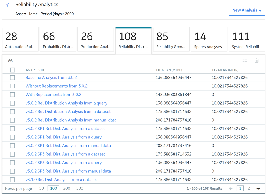
  2. Select the Reliability Distribution tab.

    A list of Reliability Distribution Analyses available in the database appears.


  3. Select the Reliability Distribution Analysis whose details you want to view.

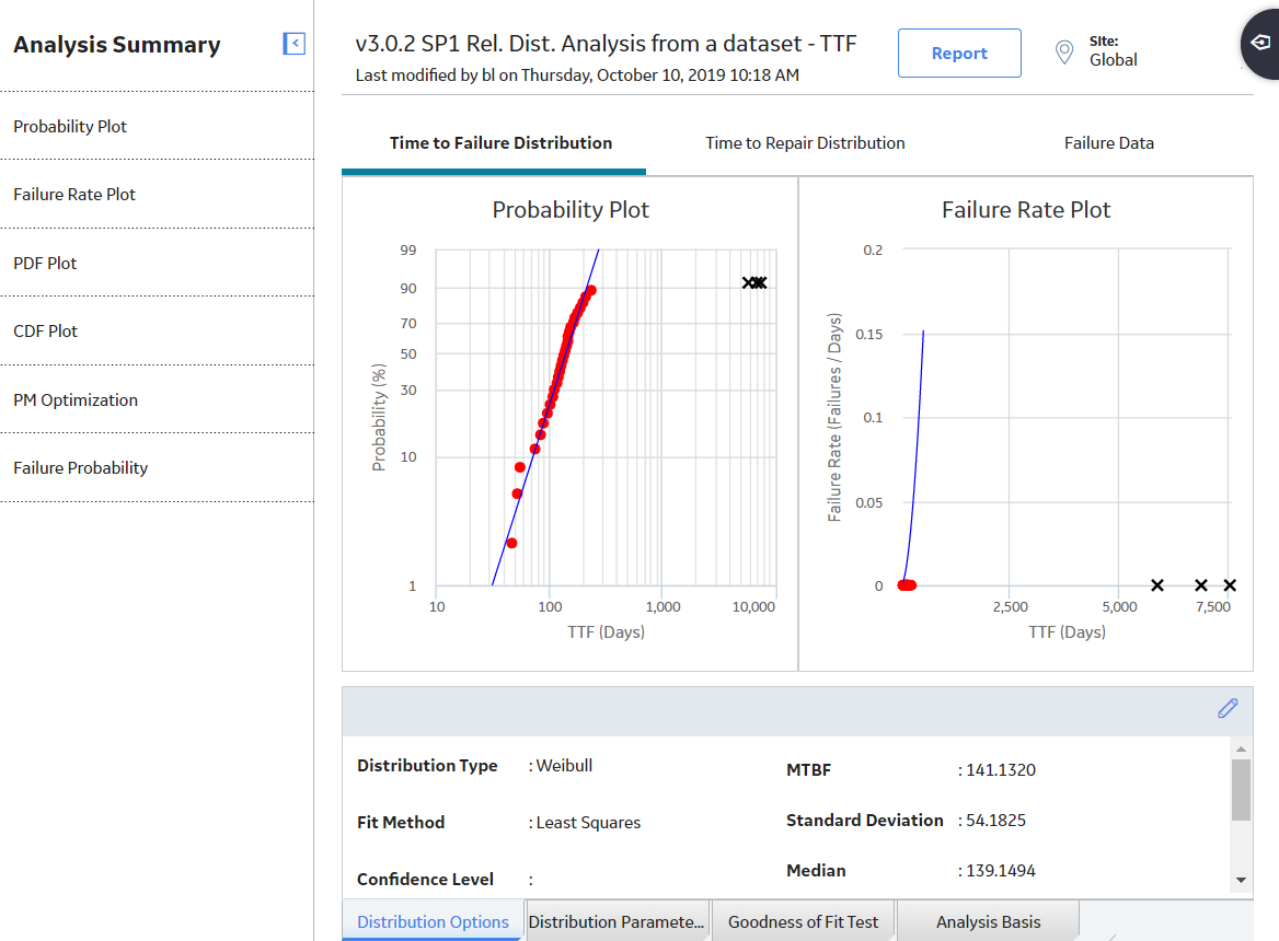
    The Analysis Summary workspace for the selected analysis appears, displaying the following sections:

    • Time to Failure Distribution: Provides a summary of details for the Time to Failure (TTF) distribution, which calculates the expected time to failure for a non-repairable system (i.e., the failed component must be replaced). This is based on the time between when the component or group of components was placed into service and when failure(s) occur. The period which is being analyzed can end at a fixed date or time, or after a fixed number of failures have taken place. TTF may be expressed as days, hours, cycles, units processed, and so on. This section also displays the Probability Plot and Failure Rate Plot.
    • Time to Repair Distribution: Provides a summary of the details for the Time to Repair (TTR) distribution, which calculates the time it took to repair an asset. This time is generally referred to as the time from when an item fails to when it is returned to productive service. This section also displays the Probability Plot and Failure Rate Plot.
    • Failure Data: Displays the failure history by asset in a chart.

    The Analysis Summary workspace contains the following sections at the bottom of the workspace:

    Note: If Time to Failure Distribution tab is selected, the bottom section displays information associated with the Time to Failure Distribution. If Time to Repair Distribution tab is selected, the bottom section displays information associated with Time to Repair Distribution.
    • Distribution Options : Contains the summary of distribution properties for the selected Reliability Distribution Analysis and allows you to modify these properties.
    • Distribution Parameters: Contains the distribution parameters, which are determined by the distribution type.
    • Goodness of Fit Test: Contains the results of the Goodness of Fit (GOF) test and includes the Statistic, P-Value and Passed fields.
    • Analysis Basis: Displays the number of failures contained in the Failure Data that were used to generate MTBF, the number of those failures from the data that were censored when the calculations were last performed, and the number of pieces of equipment contained in the Failure Data. The Failure Type that was selected when creating the analysis is also listed in this section.

      • If the analysis is based on the Failures With Replacements failure type, the following information is displayed: Components are always replaced after each failure.
      • If the analysis is based on the Failures Without Replacements failure type, the following information is displayed: Components are not automatically replaced after each failure.

    The left pane contains the following tabs:

    • Probability Plot : Contains the Probability plot for the selected analysis.
    • Failure Rate Plot : Contains the Failure Rate plot for the selected analysis.
    • PDF Plot: Contains the Probability Density Function plot for the selected analysis.
    • CDF Plot: Contains the Cumulative Distribution Function plot for the selected analysis.
    • PM optimization : Contains the optimal preventive maintenance interval and a graphical plot of the Planned Cost, Unplanned Cost, and Total Cost if a PM Optimization has been previously performed. The Optimal Value inflection point is identified on the total cost curve.
    • Failure Probability : Contains the Failure Probability information in a grid, which is calculated by the system using the Future Age that you specify and the information available for the Distribution Analysis.


Access Multiple Reliability Distribution Analyses

About This Task

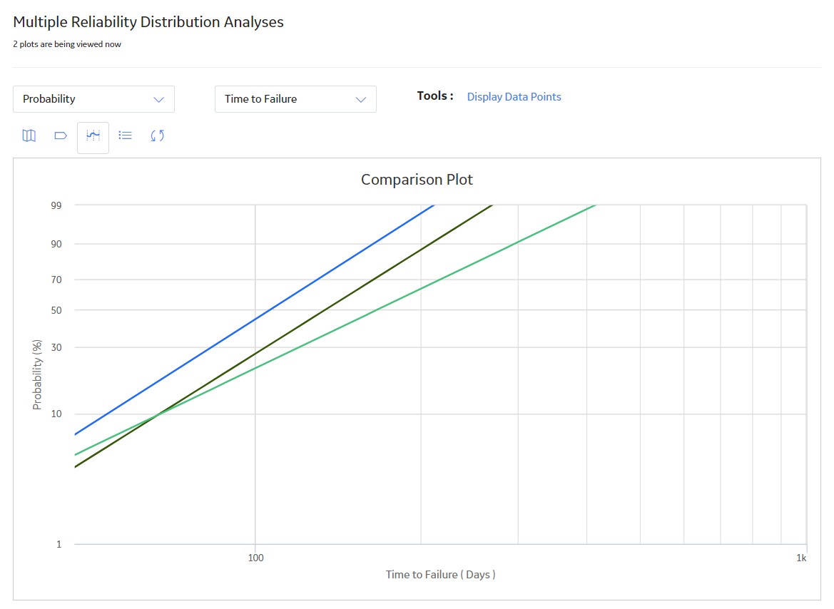
You can access multiple Reliability Distribution Analyses and compare multiple plots for the selected analyses. You cannot modify the details of the analyses based on which the Comparison Plot is generated.

Procedure

  1. Access the RA Overview page.
  2. Select the Reliability Distribution tab.

    A list of Reliability Distribution Analyses available in the database appears.


  3. Select two or more Reliability Distribution Analyses whose plots you want to compare.
    Note: You can select up to 20 analyses to compare plots.
  4. In the upper-right corner of the grid, select .

    The Multiple Reliability Distribution Analyses page appears, displaying the Comparison Plot. By default, Probability plot for the selected analyses appears. You can also view the following types of plots:

    By default, the plots appear in the Time to Failure Distribution format. You can also view multiple plots in the Time to Repair Distribution format.


Create a Reliability Distribution Analysis From an Existing Query or Dataset

Procedure

  1. Access the RA Overview page.
  2. In the upper-right corner of the page, select New Analysis, and then select Reliability Distribution.

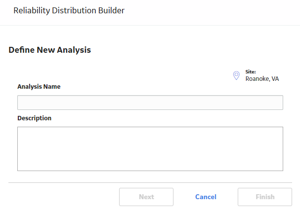
    The Reliability Distribution Builder window appears, displaying the Define New Analysis screen.


    Note: All required information is provided, but for additional information, consult the Distribution Analysis Families topic.
  3. Enter values in the Analysis Name and Description boxes for the new analysis, and then select Next.

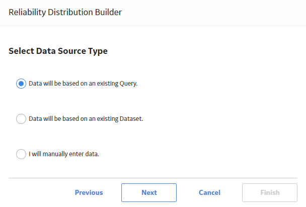
    The Select Data Source Type screen appears. The Data will be based on an existing Query option is selected by default.


  4. If you want to load data using an existing query, select Next.

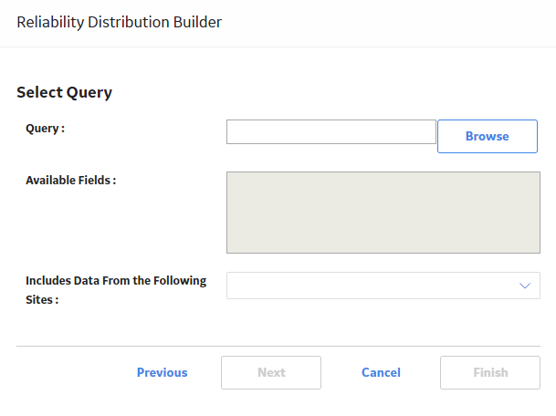
    The Select Query screen appears.


    -or-

    If you want to load data using an existing dataset, select Data will be based on an existing Dataset, and then select Next.

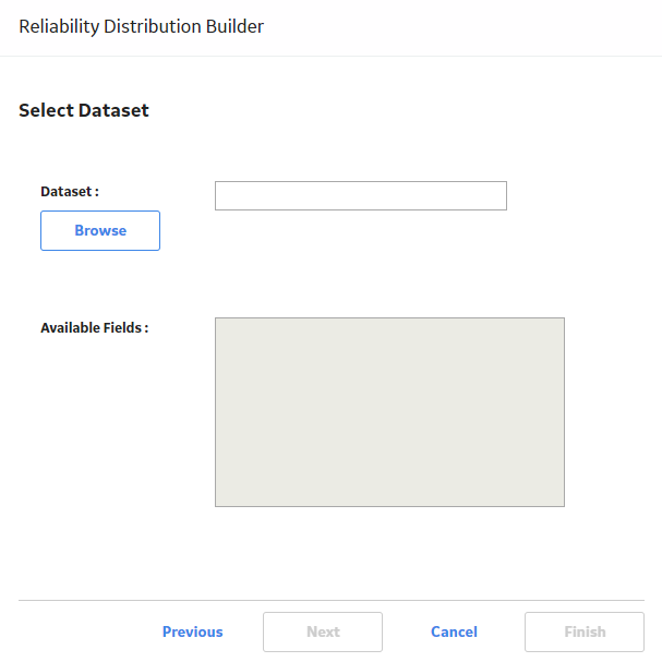
    The Select Dataset screen appears.


  5. Select Browse to search for an existing query or dataset in the APM Catalog.

    The Select a query from the catalog or Select a dataset from the catalog window appears, depending on whether you selected Data will be based on an existing Query or Data will be based on an existing Dataset in the previous step.

  6. Select the required query or dataset, and then select Open.

    The complete path to the query or dataset is displayed in the Query or Dataset box. The fields that exist for the selected query or dataset appear in the Available Fields list.

  7. In the Includes Data From the Following Sites list, select the site(s) whose data from which you want to create an analysis.
    If you are creating an analysis in a database that has only one site stored in the Site Reference family, then the Includes Data From the Following Sites list will not appear on the Select Query screen.
  8. Select Next.

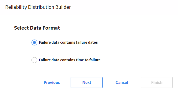
    The Select Data Format screen appears.


  9. If the failure data contains failure dates, select Failure data contains failure dates, and then select Next.

    -or-

    If the failure data contains numbers representing the time to failure, select Failure data contains time to failure, and then select Next.

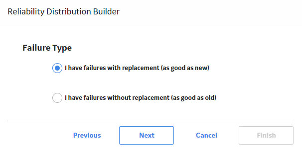
    The Failure Type screen appears.


  10. If the piece of equipment is replaced after each failure, select I have failures with replacement (as good as new) , and then select Next.

    -or-

    If the piece of equipment is not replaced after each failure, select I have failures without replacement (as good as old), and then select Next. Select this option if a failure does not require replacement of the entire unit (e.g., for heat exchangers, boiler tubes, or piping).

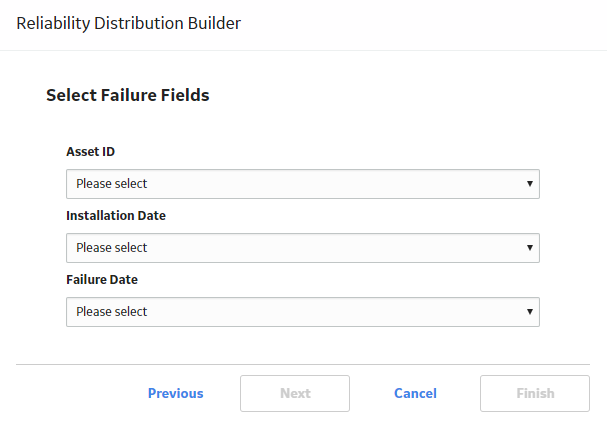
    The Select Failure Fields screen appears. This screen may look different depending on the option that you selected on the previous screen.

    The following image shows the screen that appears if you select I have failures with replacement (as good as new):


  11. Specify values in the fields:
    • In the Asset ID list, select the name of the field that contains the IDs of the failed entities. This is a required field and must be a character field.
    • In the Installation Date list, select the name of the field that contains the installation date, which is the date when the piece of equipment was installed. This is an optional field.
    • In the Failure Date list, select the name of the field that contains the failure date, which is the date on which the failure events occurred (e.g., the Out of Service date). This is a required field.
  12. If you selected I have failures without replacement (as good as old), enter values in the following additional fields, which appear only when you have made this selection:
    • Number of Subcomponents: The name of the field that contains the number of subcomponents contained by the piece of equipment that you selected in the Asset ID field.

      Note: If this field is not mapped, a warning message will appear, indicating that the number of subcomponents must be entered for every analyzed piece of equipment. You must enter those values in the Assets section of the Reliability Distribution Failure Data window to include non-failed elements. Failure probability cannot be calculated if this value is left blank.
    • Number of Failures: The name of the field that contains the number of failed elements at each failure event.
    • Replacement?: The field that indicates whether replacement is made following each equipment failure. It must be mapped to a field of the type Logical. A replacement causes the entire piece of equipment to be renewed, thus resetting calculation of the time to failure.
  13. If you selected a query or dataset that includes downtime data, select Next.

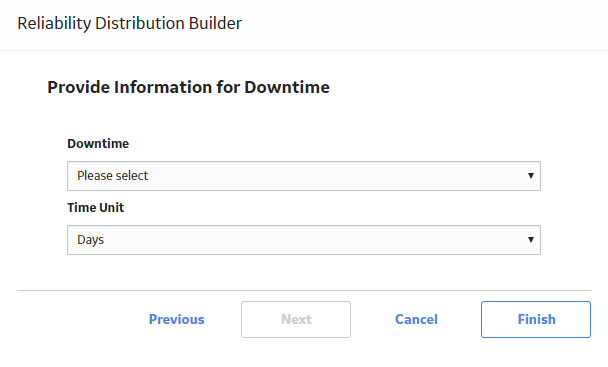
    The Provide Information for Downtime screen appears.


    -or-

    If you selected a query or dataset that does not include downtime data, select Finish, and then skip to the end of these instructions.

  14. In the Downtime Field list, select the necessary field (e.g., Total Time to Repair). This is an optional field, and the value entered must be numeric.
  15. In the Time Units list, select the time units associated with downtime from the following options:
    • Hours
    • Days
    • Weeks
    • Months
    • Quarters
    • Years
    Note: The time units that you select here will apply to downtime only. Operating time will be set by default to days. After the analysis has been created, you can change the units for both downtime and operating time.
  16. Select Finish.

    The APM system generates the analysis. The Reliability Distribution Analysis page appears, displaying the results of the analysis.

Create a Reliability Distribution Analysis From Manually Entered Data

Procedure

  1. Access the RA Overview page.
  2. In the upper-right corner, select New Analysis, and then select Reliability Distribution.

    The Reliability Distribution Builder window appears, displaying the Define New Analysis screen.


    Note: All required information is provided, but for additional information, consult the Distribution Analysis Families topic.
  3. Enter values in the Analysis Name and Description fields for the new analysis, and then select Next.

    The Select Data Source Type screen appears.


  4. Select I will manually enter failure data, and then select Next.

    The Select Data Format screen appears.


  5. If the failure data contains failure dates, select Failure data contains failure dates.

    -or-

    If the failure data contains numbers representing the time to failure, select Failure data contains time to failure.

  6. Select Next.

    The Failure Type screen appears.


  7. If the piece of equipment is replaced after each failure, select I have failures with replacement (as good as new).

    -or-

    If the piece of equipment is not replaced after each failure, select I have failures without replacement (as good as old). Select this option if a failure does not require replacement of the entire unit (e.g., for heat exchangers, boiler tubes, or piping).

  8. Select Finish.

    The Reliability Distribution Data window appears, displaying the Failures and Assets tabs. This screen may look different depending on the option that you selected on the previous screen.

  9. Enter information about the Failures and Assets that you want to include in the analysis. When you provide the information, consider the following:
    • A minimum of three failure datapoints are needed to perform a calculation.
    • If you enter downtime values that exceed the next failure date, the APM system will highlight the downtime values on the Reliability Distribution Failure Data window. When you close the Reliability Distribution Failure Data window, an error message appears in the Analysis Information section.
    • Days will be assumed to be the units for both downtime and operating time for the data that you enter. After you create the analysis, you can change the time units.
    Tip: You can add more rows of data by selecting Add at the bottom of the Reliability Distribution Failure Data window. You can remove any row of data by selecting Remove next to the row of data that you want to remove.
  10. Select OK.

    The Reliability Distribution Analysis page appears, displaying the results of the analysis.

Change the Distribution Type of a Reliability Distribution Analysis

About This Task

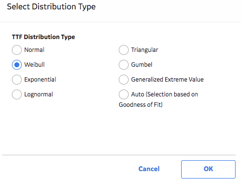
When you create a Reliability Distribution Analysis, the distribution type is set to Weibull by default. After the analysis is created, you can change the distribution type to one of the following:

Note: Select Auto if you want the APM system to select the appropriate Distribution Type based on the results of the Goodness of Fit test.

You can change the Distribution Type in the Analysis Summary workspace or from one of the plot tabs in the left pane.

Procedure

  1. Access a Reliability Distribution Analysis for which you want to modify the Distribution Type.
  2. If you want to change the distribution type in the Analysis Summary workspace:
    1. Select the Time to Failure Distribution tab.
    2. In the bottom section, select Distribution Options, and then select .

      The Distribution Type list is enabled.

    3. In the Distribution Type list, select the necessary Distribution Type, and then select .

      The analysis is recalculated based on the selected Distribution Type.

    -or-

    If you want to change the Distribution Type from one of the plot tabs (e.g., Probability Plot tab):

    1. In the left pane, select the Probability Plot tab.

      The Probability Plot appears in the workspace.

      Note: You can also change the Distribution Type via the PDF Plot tab, Failure Rate Plot tab, CDF Plot tab, or the Failure Probability tab.
    2. In the upper-right corner of the workspace, select Distribution Options, and then select Distribution Type.

      The Select Distribution Type window appears.


    3. Select the necessary Distribution Type, and then select OK.

      The analysis is recalculated based on the selected Distribution Type.

Change the Distribution Parameters in a Reliability Distribution Analysis

About This Task

This topic describes how to modify the values of the distribution parameters in a Reliability Distribution Analysis.

You can change the distribution parameters from the Analysis Summary workspace or from any of the plot tabs in the left pane.

Procedure

  1. Access a Reliability Distribution Analysis for which you want to modify the Distribution Parameters.
  2. If you want to modify the values of the Distribution Parameters from the Analysis Summary workspace:
    1. In the bottom section, select Distribution Parameters, and then select .

      The Calculate check boxes appear below each of the parameters.

    2. Clear the Calculate check box next to the parameter(s) whose value you want to modify.

      The parameter field(s) are enabled.

    3. Enter the desired value for the parameter.
    4. Select .
      Note: If you reselect the Calculate check box after manually entering data, the manually entered data for the parameter will not be retained. If you decide not to use the parameters you entered, select , and the previous selection will be used in the calculations.

      The system recalculates the analysis based on the selected distribution parameter.

    -or-

    If you want to modify the values of the distribution parameters from one of the plot tabs (e.g., Probability Plot tab):

    1. In the left pane, select the Probability Plot tab.

      The Probability Plot appears in the workspace.

      Note: You can also change distribution parameter via the PDF Plot, CDF Plot, and Failure Rate Plot tabs.
    2. In the upper-right corner of the workspace, select Distribution Options, and then select Distribution Parameters.

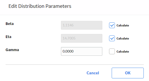
      The Edit Distribution Parameters window appears.


    3. Clear the Calculate check box next to the parameter(s) whose value you want to modify.

      The parameter field(s) are enabled.

    4. Enter the desired value for the parameter, and then select OK.
      Note: If you reselect the Calculate check box after manually entering data, the manually entered data for the parameter will not be retained. If you decide not to use the parameters you entered, select Cancel, and the previous selection will be used in the calculations.

      The system recalculates the analysis based on the selected distribution parameter.

Change the Fit Method of a Reliability Distribution Analysis

About This Task

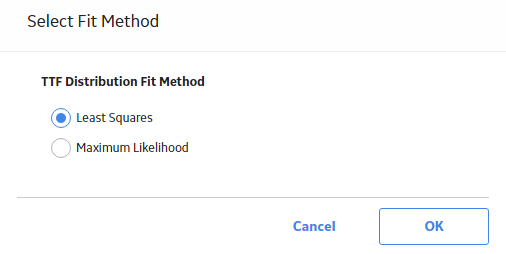
The Kolmogorov-Smirnov test is a Goodness of Fit (GOF) test applied to Reliability Distribution Analyses to determine how well the data fits the analytical curve. When you create an analysis, by default, the fit method is set to Least Squares.

After the analysis is created, you can modify the fit method to one of the following:

  • Least Squares: A curve-fitting estimation method that relies on linear regression techniques to estimate the parameters for the distribution.
  • Maximum Likelihood Estimators: A curve-fitting estimation method that maximizes the likelihood function for a given population. This method includes a survivor function that estimates changes in reliability as the piece of equipment or location survives beyond a certain age.

You can change the fit method in the Analysis Summary workspace or after selecting any of the plot tabs in the left pane.
Procedure

  1. Access a Reliability Distribution Analysis for which you want to modify the fit method.
  2. If you want to change the fit method from the Analysis Summary workspace:
    1. In the bottom section, select Distribution Options, and then select .

      The Fit Method list is enabled.

    2. From the Fit Method list, select the desired fit method, and then select .

      The analysis is recalculated based on the selected fit method.

    -or-

    If you want to change the fit method after selecting one of the plot tabs (e.g., Probability Plot tab):

    1. In the left pane, select the Probability Plot tab.

      The Probability Plot appears in the workspace.

    2. In the upper-right corner of the workspace, select Distribution Options, and then select Fit Method.

      The Select Fit Method window appears.


    3. Select the desired fit method, and then select OK.

      The analysis is recalculated based on the selected fit method.

Delete a Reliability Distribution Analysis

Procedure

  1. Access the RA Overview page.
  2. Select the Reliability Distribution tab.

    A list of Reliability Distribution Analyses available in the database appears.


  3. Select the row containing the Reliability Distribution Analysis that you want to delete, and then select .

    The Delete Reliability Distribution Analysis dialog box appears, asking you to confirm that you want to delete the selected analysis.

  4. Select Yes.

    The selected analysis is deleted.