Probability Distribution Analyses
About Probability Distribution Analysis
Probability Distribution Analysis allows you to describe the Time to Failure (TTF) as a statistical distribution, which usually is characterized by a specific pattern.
Based on a query, dataset, or data that you manually enter, you can use an independent variable to generate a Probability Distribution Analysis. APM Reliability supports four Distribution types:
About Data Censoring in a Probability Distribution Analysis
Probability Distribution Analysis supports the functionality of censoring, which accounts for the period of time from the last failure date to the analysis end date. You can censor or ignore datapoints in a Probability Distribution Analysis to estimate the probability when a failure might occur. Censoring is based on failure modes.
Censoring a datapoint means that the datapoint is excluded as a failure but included in the operating time of the Asset. If you select the Censored check box, the data in the selected row is excluded. When you create a Probability Distribution Analysis using a query or dataset as the data source, the APM system automatically censors time values from the beginning of the Analysis Period to the first event and the time value from the last event to the end of the analysis. After the calculations for the analysis have been performed, each time that the query or dataset is refreshed, the failure data will be automatically censored.
Regardless of the data source you use, you can censor any failure data. Consider the following:
- For Maximum Likelihood Estimators (MLE), the maximum number of censored datapoints is one (1) less than the total number of datapoints.
- For Least Squares estimation, the maximum number of censored datapoints is two (2) less than the total number of datapoints.
Pump Failure
Assume that you want to determine the reasons for a pump failure.
A pump might have failed due to multiple reasons, such as rusted part, motor overheating, insufficient power supply, or power outage. Each of these reasons will have its own specific failure rate and probability density function. To determine the failure rate of "motor overheating," you must censor all other failure modes from the analysis.
Further, motor overheating might be caused due to multiple reasons, such as improper operation, improper application, and improper maintenance. The censoring feature allows you to separate the failure modes, and determine which is the dominant failure mode. Based on this information, you can decide what is needed to improve the motor performance.
Access a Probability Distribution Analysis
Procedure
About Probability Plot
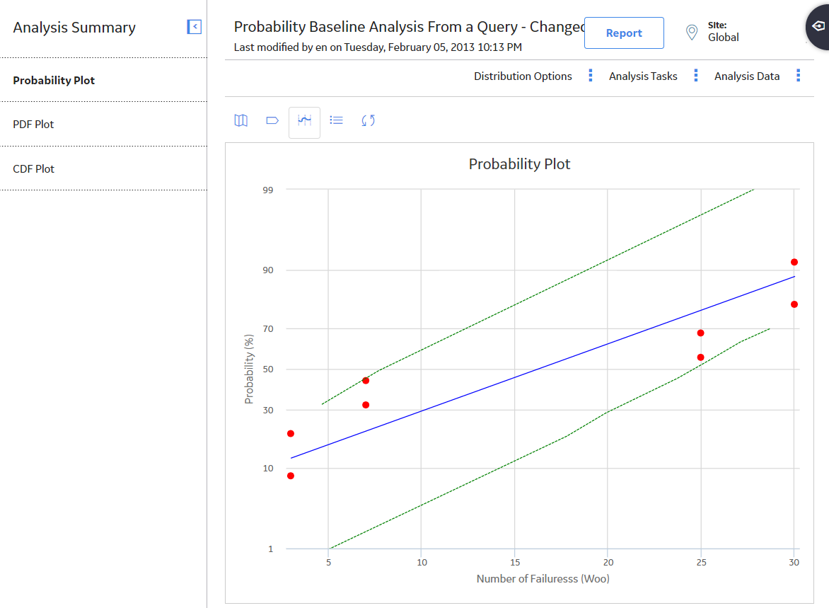
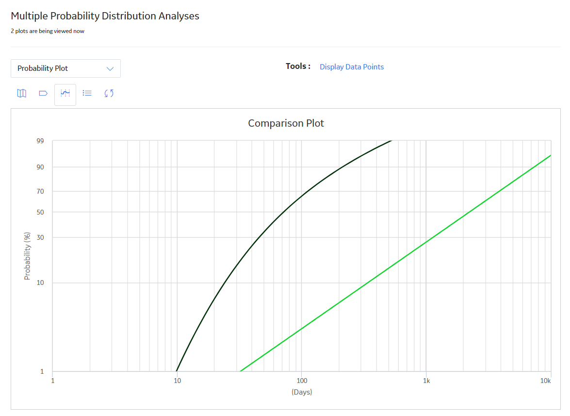
The Probability Plot is a log-log plot with data overlay and confidence limits that graphically displays the probability (expressed as a percentage) of each possible value of the random variable (CDF Occurrence % vs. time). CDF Occurrence % used here is numerically equal to the value from the cumulative distribution.
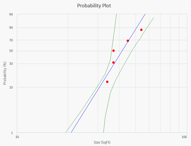
The Probability Plot shows the same data as the CDF plot, just represented in a log-log format. The log-log format reflects the standard technique for representing Weibull Distribution. Log-log format Data overlay gives a visual estimate of Goodness of Fit (GOF). Data overlay also gives clues to the presence of multiple failure modes. If a single or multiple inflection points exist in the data, then there is a possibility of multiple failure modes.
Graph Features
While accessing a Probability Plot, you can:
-
Hover or tap on any datapoint to view the coordinates and the details of a datapoint.
- For an Estimated datapoint, you can view the type of distribution, the distribution parameters, and the value of R-Squared.
- For an Observed datapoint, you can view the name and the value of Variable.
-
Click or double-tap on any observed datapoint to view the data on the Distribution Data window.
- Censor a datapoint.
- Customize the appearance of the plot by using standard graph features.
- Customize the data displayed in the graph by adjusting the x-axes to vary the display range.
About Failure Rate Plot
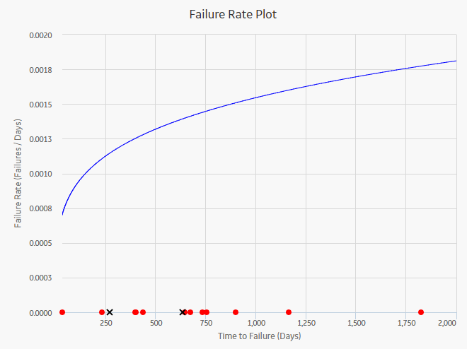
The Failure Rate Plot shows the instantaneous failure rate of the population.
- If the function is increasing, then equipment is wearing out.
- If the function is decreasing, then equipment is subject to infant mortality.
Graph Features
When you access a Failure Rate Plot, APM displays auto-censored datapoints that represent the life between the last date of the failure and the end of the analysis.
While viewing a Failure Rate Plot, you can:
- Hover or tap on any datapoint to view the coordinates and the details of a datapoint.
- For an Estimated datapoint, you can view the type of distribution, the distribution parameters, and the value of R-Squared.
- For an Observed datapoint, you can view the name and the value of Variable.
- Select an observed datapoint to open the Point Information window. You can then select Go To Editor to view data.
- Censor a datapoint.
- Customize the appearance of the graph by using standard graph features.
About PDF Plot
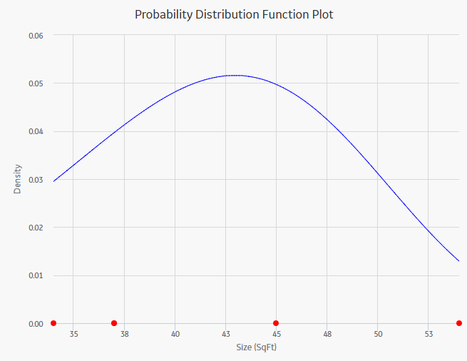
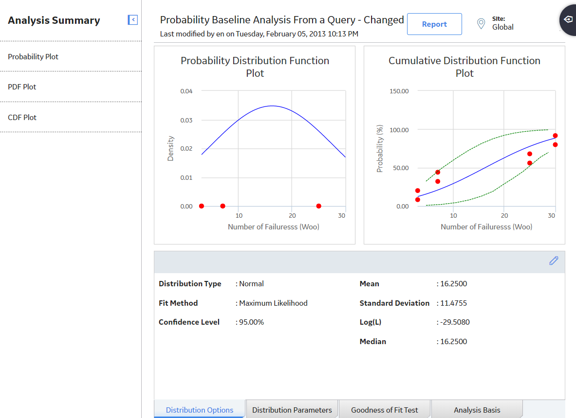
The Probability Density Function (PDF) plot is a lin-lin plot that counts the number of failures (or any other data) between certain time periods, creating a curve fit that estimates how many failures (failure data or any other data) you can expect to occur at a given point of time. This plot shows Density vs. Size. The term Density is used here with failure data to describe the size of the population that failed at the particular value of size (SqFt). A PDF plot helps you to answer a question such as, "What is the chance of a member of the population failing at exactly the time in question?"
Graph Features
While accessing a PDF plot, you can:
- Hover or tap on any datapoint to view the coordinates and the details of a datapoint.
- For an Estimated datapoint, you can view the type of distribution, the distribution parameters, and the value of R-Squared.
- For an Observed datapoint, you can view the name and the value of Variable.
- Click or double-tap on any observed datapoint to view the data on the Distribution Data window.
- Censor a datapoint.
- Customize the appearance of the plot by using standard graph features.
- Customize the data displayed in the graph by adjusting the x-axes to vary the display range.
About CDF Plot
The Cumulative Distribution Function (CDF) plot is a lin-lin plot with data overlay and confidence limits. It shows the cumulative density of any data set over time (i.e., Probability vs. size). The term Probability is used in this instance to describe the size of the total population that will fail (failure data or any other data) by size (SqFt).
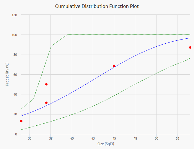
CDF plot answers a different question than PDF. For example, "What is the probability of failure at Size (SqFt)?" The CDF curve is the area under the PDF curve. The CDF accumulates all probability of failure up to the point in time in question. Since the number of failures increases with increasing size, the slope of the curve is always positive, always increasing.
Graph Features
While accessing a CDF plot, you can:
- Hover or tap on any datapoint to view the coordinates and the details of a datapoint.
- For an Estimated datapoint, you can view the type of distribution, the distribution parameters, and the value of R-Squared.
- For an Observed datapoint, you can view the name and the value of Variable.
- Click or double-tap on any observed datapoint to view the data on the Distribution Data window.
- Censor a datapoint.
- Customize the appearance of the plot by using standard graph features.
- Customize the data displayed in the graph by adjusting the x-axes to vary the display range.
About Preventive Maintenance Optimization
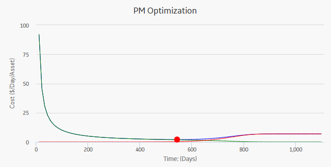
Preventative Maintenance (PM) Optimization uses the results of a Reliability Distribution Analysis to measure the optimum time to perform a Planned (Restorative) Maintenance (PM) procedure on a piece of equipment. PM optimization does not calculate minor maintenance schedules but determines the optimal time to perform major repairs or replace a piece of equipment until there is a minimal amount of cost and risk. PM optimization is only valid for wear-out failure modes and will not give accurate results for a Weibull analysis where Beta is less than 1.
Details
A PM optimization is composed of the following steps:
- The calculation model is configured to acquire the necessary parameters, including Mean Time Between Failures (MTBF). MTBF is used to determine the probability that a piece of equipment will fail.
- The cost ratio is determined. This ratio is the cost of planned Preventative Maintenance (PM) events versus the cost of unplanned maintenance events. You can manually enter the cost or select an existing query as the source of the cost data.
- Based on the MTBF and the calculation of the ratios, the APM system estimates the optimum time (interval) to maintain equipment. The cost per piece of equipment based on the Optimized Preventative Maintenance Interval is also displayed.
- The APM system creates optimization graphs, which gives the analyst the optimum time to conduct a repair or overhaul based upon the ratio of planned to unplanned repair costs. This ensures that repairs are conducted in a cost-effective manner, minimizing risk while maximizing time in service.
The limitation to using a PM optimization is it will always give a result for the statistical distribution on which it is based. This does not mean that it will always make sense to do a PM at the interval specified. In particular, design flaws that manifest themselves as poor reliability can more effectively be addressed through redesign rather than PM.
Collect Data for Probability Distribution Analysis
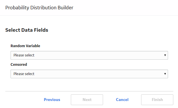
To create a Probability Distribution Analysis, you must select the field that contains the value that you want to analyze.
The following table shows the typical data needed to build and analyze Probability Distribution Analyses.
| Data Required | Data Type | Description | Behavior and Usage |
|---|---|---|---|
|
Censored | Logical |
As needed, select the field to provide censoring information. Select the field from the data source that contains a value that indicates censored values. |
This field is optional. |
|
Random Variable | Character |
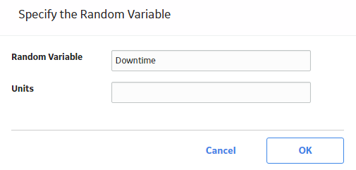
If the data source is a query, the name of the random variable and the units of measure will be pre-populated based on the selection you made in the Value field on the previous screen. If you selected a different data source, type the name of the random variable in the Random Variable field and the units of measure for the random variable in the Units field. |
This field is optional.
|
|
Units | Character |
Select the units of measure for the random variable. |
This field is optional. |
|
Value | Numeric |
Select the field that contains the value you want to analyze. |
This is a required field. |
Access Multiple Probability Distribution Analyses
About This Task
You can access multiple Probability Distribution Analyses and compare multiple plots for the selected analyses. You cannot modify the details of the analyses based on which the Comparison Plot is generated.
Procedure
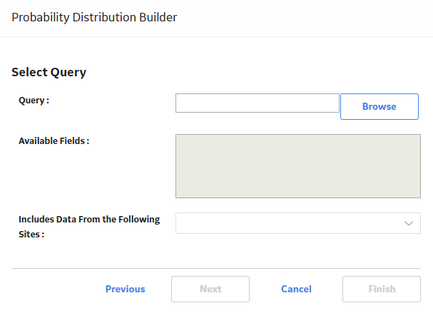
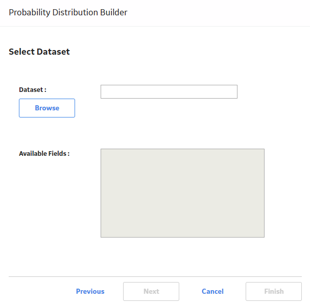
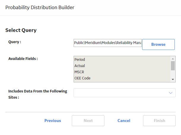
Create a Probability Distribution from an Existing Query or Dataset
Procedure
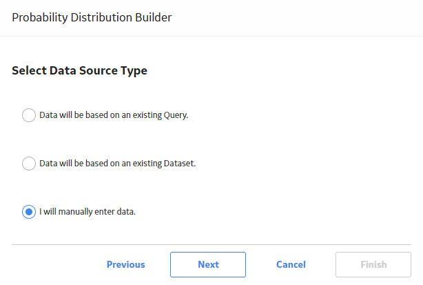
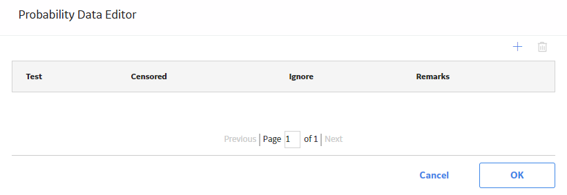
Create a Probability Distribution from Manually Entered Data
Procedure
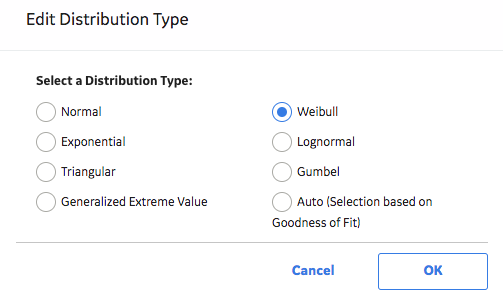
Change the Distribution Type of a Probability Distribution Analysis
About This Task
When you create a Probability Distribution Analysis, the Distribution Type is set to Weibull by default. After the analysis is created, you can change the Distribution Type to one of the following:
You can change the Distribution Type from the Analysis Summary workspace or from any of the plot tabs in the left pane.
Procedure
Change the Distribution Parameters in a Probability Distribution Analysis
About This Task
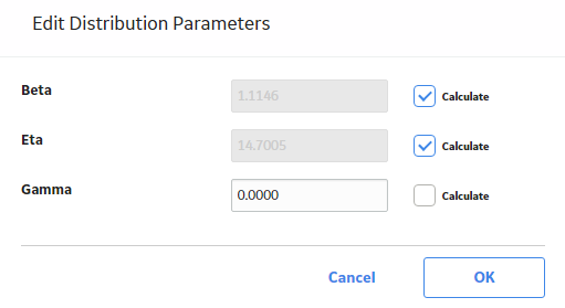
This topic describes how to modify the values of the distribution parameters in a Probability Distribution Analysis.
You can change the distribution parameters from the Analysis Summary workspace or from any of the plot tabs in the left pane.
Procedure
Change the Fit Method of a Probability Distribution Analysis
About This Task
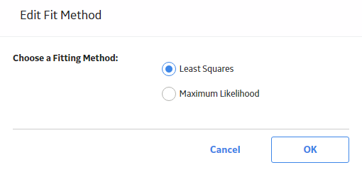
The Kolmogorov-Smirnov test is a Goodness of Fit (GOF) test applied to a Probability Distribution Analysis to determine how well the data fits the analytical curve. When you create an analysis, the fit method is set to Least Squares by default.
After the analysis is created, you can modify the fit method to one of the following:
- Least Squares: A curve-fitting estimation method that relies on linear regression techniques to estimate the parameters for the distribution.
- Maximum Likelihood Estimators: A curve-fitting estimation method that maximizes the likelihood function for a given population. This method includes a survivor function that estimates changes in reliability as the piece of equipment or location survives beyond a certain age.
You can change the fit method from the Analysis Summary workspace or from any of the plot tabs in the left pane.
Procedure
Modify the Confidence Level for a Probability Distribution Analysis
About This Task
The Confidence Level specifies how the optimistic and realistic scenarios will be selected in a Monte Carlo Simulation for TTR Distributions in an analysis. The Confidence Level indicates whether the distribution is within the confidence limits or not. The default Confidence Level for an analysis is 90 percent.
You can modify the Confidence Level from the Analysis Summary workspace or from any of the plot tabs in the left pane.
Procedure
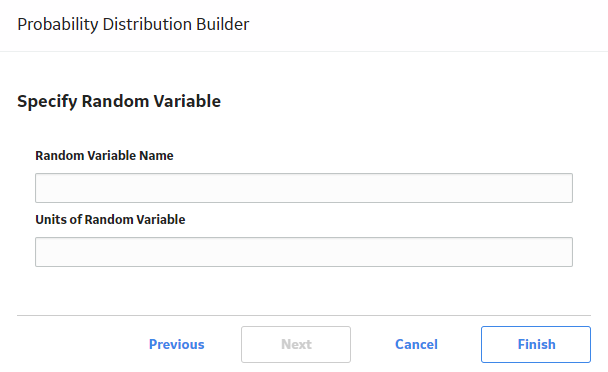
Modify the Random Variable and Specify Units for a Probability Distribution Analysis
Procedure
Rename a Probability Distribution Analysis
Procedure
Access the Source Data for a Probability Distribution Analysis
Procedure
Modify Data in a Probability Distribution Analysis
Procedure
Results
- For an analysis that is based on manually entered data, the changes that you make via the Probability Distribution Data window will be saved for the analysis.
- For an analysis that is based on a query or a dataset:
- The query or dataset will not be modified with the updated data. Additionally, any record returned by the query will not be updated with your changes. The changes will be saved to the analysis only.
- After you modify the data and save the analysis, the modified data will appear each time you open the analysis. If you want to revert to the original data, you can reload the original data to the analysis. In addition, if a query or dataset has changed in the database, you can reload the data in order for your analysis to contain those changes.
Reload Analysis Data in a Probability Distribution Analysis
About This Task
When you create and save an analysis that is based on a query or dataset, the APM system takes a snapshot of the data that exists at the time of creation and saves it along with the analysis. When you open an existing analysis, the APM system loads the data that was last saved with the analysis. This means that any changes to the underlying query or dataset will not be reflected automatically when you open an existing analysis.
If you want to refresh an analysis based upon changes to the underlying query or dataset or to load new data that has been added since the analysis was last saved (e.g., the analysis is based on a query that retrieves failures for a piece of equipment or location, and a new failure record has been added to the database), you will need to reload the analysis manually after opening it. When you reload the data, any manual changes made to the analysis data set will be deleted.
Procedure
Censor Data in a Probability Distribution Analysis
Procedure
Delete a Probability Distribution Analysis
Procedure
Access Probability Distribution Report
Procedure
About Probability Distribution Report
The baseline APM database includes the Probability Distribution report, which you can use to view a summary of the results of a Probability Distribution Analysis.
The Probability Distribution report is built from the following Catalog items:
- The subreport, SubReportProbDist, which is stored in the Catalog folder \\Public\Meridium\Modules\Reliability Manager\Reports.
- The supporting queries that supply data in the main report and subreport, which are stored in the Catalog folder \\Public\Meridium\Modules\Reliability Manager\Reports. The following supporting queries are available:
- ProbabilityDistributionQuery
- Weibull Distribution Query
- Lognormal Distribution Query
- Normal Distribution Query
- Exponential Distribution Query
Throughout this documentation, we refer to the main report, the subreport, and the supporting queries collectively as the Probability Distribution report.
The Probability Distribution report contains a prompt on the ENTY KEY and Distribution Type fields in the Distribution family. When you run the Probability Distribution report via the Probability Distribution module, the ENTY KEY and Distribution Type of the Distribution record associated with the current analysis is passed automatically to the prompt, and the results for the current Probability Distribution Analysis are displayed. If you run the main report or any of the queries in the preceding list directly from the Catalog, however, you will need to supply the ENTY KEY and Distribution Type of a Distribution record manually to retrieve results. The subreport (i.e., Catalog item SubReportProbDist) cannot be run directly from the Catalog.
Analysis Summary Section
The Analysis Summary section of the Probability Distribution report displays information that is stored in a Distribution record. Distribution records are categorized into one of four Distribution subfamilies: Exponential, Lognormal, Normal, or Weibull.
The following table lists each item in the Analysis Summary section and the corresponding Distribution record field whose data is displayed in the report.
| Report Item | Distribution record |
|---|---|
| Analysis Name | Analysis ID |
| Analysis Description | Short Description |
| Random Variable | Random Variable Field |
| Units | Units |
| Last Modified | LAST UPDT DT |
| Modified By |
LAST UPBY SEUS KEY Note: The name of the Security User associated with this value is displayed in the report.
|
Statistical Distribution Information Section
The Statistical Distribution Information section of the Probability Distribution report displays information that is stored in the Distribution record (i.e., Exponential, Lognormal, Normal, or Weibull record).
The following subsections are displayed within the Statistical Distribution Information section:
The Distribution Type subsection displays information that is stored in the Distribution record. Throughout the documentation, we will refer to this subsection as the Distribution subsection.
The following table lists each item in the Distribution subsection and the corresponding Distribution record field whose data is displayed in the report.
| Report Item | Distribution Field |
|---|---|
| Distribution Type |
Distribution Type |
| Fit Method |
Fit Method |
| Use Confidence |
Use Confidence |
| Confidence Level | Confidence Level |
| Mean | Mean |
| Standard Deviation | Standard Deviation |
| Median |
Median |
| R2 | R-Squared |
The Parameters subsection contains information stored in the Distribution record. The type of information that appears in the Parameters subsection depends on the distribution type (i.e., Weibull, Lognormal, Exponential, or Normal).
The following table lists each item in the Parameters subsection for a Weibull record whose data is displayed in the report. One row is displayed for each of the following field captions: Beta, Eta, and Gamma.
| Report Item | Weibull Field |
|---|---|
| Beta | |
| Value |
Beta |
| Low |
Beta Low |
| High | Beta High |
| Calculated | Beta Fixed |
| Eta | |
| Value | Eta |
| Low | Eta Low |
| High |
Eta High |
| Calculated | Eta Fixed |
| Gamma | |
| Value | Gamma |
| Low | Gamma Low |
| High |
Gamma High |
| Calculated | Gamma Fixed |
The following table lists each item in the Parameters subsection for a Lognormal record whose data is displayed in the report. For a Lognormal record, one row is displayed for each of the following field captions: Mu, Sigma, and Gamma.
| Report Item | Lognormal Field |
|---|---|
| Mu | |
| Value |
Mu |
| Low |
Mu Low |
| High | Mu High |
| Calculated | Mu Fixed |
| Sigma | |
| Value | Sigma |
| Low | Sigma Low |
| High |
Sigma High |
| Calculated | Sigma Fixed |
| Gamma | |
| Value | Gamma |
| Low | Gamma Low |
| High |
Gamma High |
| Calculated | Gamma Fixed |
The following table lists each item in the Parameters subsection for an Exponential record whose data is displayed in the report. For an Exponential record, one row is displayed for the field caption MTBF.
| Report Item | Exponential Field |
|---|---|
| MTBF | |
| Value |
MTBF |
| Low |
MTBF Low |
| High | MTBF High |
| Calculated | MTBF Fixed |
The following table lists each item in the Parameters subsection for a Normal record whose data is displayed in the report. For a Normal record, one row is displayed for each of the following field captions: Mean, Standard Deviation.
| Report Item | Normal Field |
|---|---|
| Mean | |
| Value |
Mean |
| Low |
Mean Low |
| High | Mean High |
| Calculated | Mean Fixed |
| Standard Deviation | |
| Value | Standard Deviation |
| Low | Standard Deviation Low |
| High |
Standard Deviation High |
| Calculated | Standard Deviation Fixed |
The Goodness of Fit Test subsection displays information from the Distribution record.
The Kolmogorov-Smirnov test is the only test used to measure goodness of fit, so the Name column in the report is populated with the value Kolmogorov-Smirnov Test.
The following table lists each remaining item in the Goodness of Fit Test subsection and the Distribution record field whose data is displayed in the report.
| Report Item | Weibull Field |
|---|---|
| Statistic |
GOF Statistic |
| P-Value |
GOF P-Value |
| Passed |
Passed |
Distribution Data Section
The Distribution Data section of the Probability Distribution report displays information that is stored in the Data field in the Distribution record.
The following values are displayed in the Distribution Data section, and they are stored in the Data field in the Reliability Distribution record:
- X (i.e., the Random Variable)
- Censored
- Ignored
- Remarks
Plots Section
The Plots section of the Probability Distribution report displays the plots that are displayed on the Analysis Summary workspace or accessed via the Plots tabs in the left pane on the Probability Distribution page.
The Plots section displays the following graphs:
 .
. .
.
 , and the previous selection will be used in the calculations.