Open topic with navigation

About Results of a Reliability Distribution Analysis

After you have created a Reliability Distribution Analysis, the following options are available:

• Analysis results can include confidence intervals and parameters for the selected Distribution and goodness of fit measures.
• Distribution fitting can be done by Least Squares or Maximum Likelihood (MLE).
• The four different types of Reliability plots (Probability of Failure, Failure Rate, Probability Density Function, and Cumulative Distribution Function) can be displayed. In addition, you can select between 2 and 10 Distribution Analyses and choose to view and compare all four of the plot types for the selected analyses using the Competing Failure Plots feature.
• Reliability Distribution Analyses can support Failures without Replacement, which are needed to calculate reliability for heat exchangers, boiler tubes, piping, and other pieces of equipment where a repair does not necessarily involve changing the whole unit.
• The Preventive Maintenance Optimization calculator can utilize the results of the Distribution Analysis and allow you to input the estimated costs of an unplanned repair versus a planned repair. Based on the MTBF and the ratio of unplanned cost to planned cost, the system calculates the optimal time to maintain equipment.
• A Failure Probability calculator can utilize the results of a Distribution Analysis; based on MTBF, Beta, and the last Failure Date, the system calculates the probability of equipment failure at the time in the future that you specify. The system also provides the capability to calculate future life based upon a failure probability that the user specifies.
• Based on the analysis results, you can generate recommendations for the maintenance and reliability activities that should be executed in the future to maintain best practices in your organization.

Time to Failure

The most important piece of data for distributions is Time to Failure (TTF), which is also sometimes known as Time to Event (TTE) or Time Between Failures (TBF).

Suppose that you have the following timeline, where each number represents the amount of time that passes between failures.

Installation

5

11

23

38

16

22

44

32

Out of Service

You could fit a Weibull Distribution to this data. A Probability Density Function (PDF) is similar to a histogram of the raw TTF data:

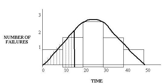
The distribution shows:

• One failure occurring between time 0 and 10.
• Two failures occurring between time 11 and 20.
• Three failures occurring between time 21 and 30.
• Two failures occurring between time 31 and 40.
• One failure occurring between time 41 and 50 (Out of service).

This type of graph counts the number of failures between certain periods. This creates a curve, which you can examine and ask: At 15 time units, how many failures can I expect to have? The answer: Between two and three failures. You are distributing the failures over the life of the equipment so that at any given point in that life, you can calculate the probability that the equipment will fail. This calculation is generated based on the area under the curve, as shown in the previous graphic. In practice, the PDF is adjusted in such a way that the area under the curve is exactly one, and the number on the y-axis represents the number of failures per time unit.

You select your historical data: other pieces of equipment by the same manufacturer, other pieces of equipment in the same location, other pieces of equipment of the same type, etc. For example, suppose that you want to buy a new pump. You could perform a Distribution Analysis on the other pumps of the same model to predict the reliability of the new pump.

Copyright © 2018 General Electric Company. All rights reserved.